APX3330 (Silva 2024)

Model and source

• Citation: Silva LL, Stratford RE, Messmann R, Kelley MR, Quinney SK. Bridging population pharmacokinetic and semimechanistic absorption modeling of APX3330. CPT Pharmacometrics Syst Pharmacol. 2024;13(1):106-117. doi:10.1002/psp4.13061.
• Description: Population pharmacokinetic model for APX3330 (E3330), a selective APE1/Ref-1 redox inhibitor, measured as total quinone in plasma after oral dosing. Two-compartment disposition with first-order absorption and an absorption lag time, fitted to 1460 plasma concentrations pooled from four Eisai studies in 49 healthy Japanese male volunteers (single dose-escalation 10-600 mg, multiple-dose 120 mg once or twice daily, and a fasted-vs-fed crossover) and one Apexian phase I study in 19 patients with advanced solid tumors dosed 120-360 mg twice daily. All disposition parameters are apparent (oral) values because absolute bioavailability was never measured. Body weight is a power-model covariate on CL/F (exponent 0.659) and V1/F (exponent 0.839) referenced to 70 kg; the oncology cohort carries a log-additive shift on CL/F, and dosing in the fed state carries a log-additive shift on the absorption lag time. Inter-individual variability is estimated on CL/F, V1/F and ka with a CL/F-V1/F correlation of 0.349, and residual error is proportional (16%). The paper’s companion GastroPlus ACAT semi-mechanistic absorption model is a commercial-platform model and is not reproduced here; see the validation vignette.
• Article: https://doi.org/10.1002/psp4.13061

APX3330 (also called E3330) is a selective inhibitor of APE1/Ref-1 that has been investigated in hepatitis, cancer, diabetic retinopathy and diabetic macular edema. It is given orally as a quinone but converts rapidly to a hydroquinone in the gastrointestinal tract. Neither bioanalytical method used in the source studies could separate the two forms – samples were oxidised before analysis – so every concentration the model was fitted to is total quinone, and every disposition parameter is an apparent (oral) quantity.

The paper pairs two modelling approaches. Only the first is packaged here:

1. A population PK model (Monolix 2019 R2), two-compartment with first-order absorption and a lag time. This is Silva_2024_apx3330.
2. A semi-mechanistic absorption model built on the advanced compartmental absorption and transit (ACAT) framework in GastroPlus 9.8, used to explain why food delays absorption. This is a commercial-platform model whose gastrointestinal physiology, transit structure and dissolution model live inside GastroPlus; the paper reports only its tuned absorption scale factors and its fasted/fed physiology set (Table S5, not in the open-access deposit). It is therefore not reproducible in rxode2 and is not packaged. See “Assumptions and deviations” below.

Which of the paper’s two parameter columns is packaged

Table 2 of Silva 2024 has two columns, “Healthy volunteers” and “Combined data”. These are the two stages of a single staged model-development strategy, not two independent models: the Methods state that “Using the final estimates from the model for healthy volunteers as initial estimates, a final model was developed to describe data from both studies.” The packaged model uses the Combined data column, the paper’s final model. Setting DIS_CANCER = 0 recovers the healthy-Japanese-volunteer reference population, whose parameters differ from the earlier stage by less than 2% (CL/F 193 vs 196 mL/h; lag time 0.401 vs 0.413 h), so nothing is lost by not carrying the intermediate stage as a separate file.

Population

The combined model was built on 1460 total-quinone plasma concentrations from 68 participants across five studies; 211 concentrations (14.45%) came from the oncology study.

The healthy-volunteer component pools four Eisai studies in 49 healthy Japanese male volunteers (mean age 25.4 years, weight 52-77 kg, mean 62.4 kg, all within +/- 20% of ideal body weight): a single-dose escalation at 10, 30, 60, 120, 180 and 240 mg; a multiple-dose study at 120 mg once or twice daily; a 120 mg fasted-versus-fed single-dose crossover; and a high single-dose study at 300, 420 and 600 mg. Individual-level data for these studies were digitised from Eisai clinical trial reports with Engauge Digitizer.

The oncology component is a single Apexian phase I study in 19 patients with advanced solid tumors dosed 120-360 mg twice daily for 22 days: 13 (68.42%) men, 84.21% White and 10.53% Hispanic, mean weight 88.3 kg. Serum albumin averaged 3.9 +/- 0.28 g/dL in patients with cancer versus 4.8 +/- 0.16 g/dL in the healthy volunteers. Baseline demographics are tabulated in the paper’s Table S3. Neither dose level nor study period was a significant covariate, indicating linear PK across the 10-600 mg range.

The same information is available programmatically via readModelDb("Silva_2024_apx3330")()$population.

Source trace

Every ini() entry in inst/modeldb/specificDrugs/Silva_2024_apx3330.R carries an in-file comment naming its source. They are collected here for review. All parameter values come from the “Combined data” column of Silva 2024 Table 2.

Equation / parameter	Value	Source location
ltlag	log(0.401) h	Table 2, row t lag (h) = 0.401 (RSE 6.92%)
lka	log(0.894) 1/h	Table 2, row k a (1/h) = 0.894 (RSE 9.47%)
lcl	log(0.193) L/h	Table 2, row CL/F (mL/h) = 193 mL/h (RSE 2.48%)
lvc	log(4.05) L	Table 2, row V 1/F (mL) = 4050 mL (RSE 2.51%)
lq	log(0.276) L/h	Table 2, row Q/F (mL/h) = 276 mL/h (RSE 4.02%)
lvp	log(4.78) L	Table 2, row V 2/F (mL) = 4780 mL (RSE 2.00%)
e_wt_cl	0.659	Table 2, row beta WT,CL (RSE 17.6%); applied via Eq. 1
e_wt_vc	0.839	Table 2, row beta WT,V1 (RSE 12.8%); applied via Eq. 1
e_cancer_cl	0.409	Table 2, row beta SubjectSource,CL (RSE 13.0%); applied via Eq. 2
e_fed_tlag	0.815	Table 2, row beta Food,tlag (RSE 13.5%); applied via Eq. 2
etalcl	0.142^2 = 0.020164	Table 2, omega CL/F = 0.142 (RSE 9.67%), an SD
etalvc	0.141^2 = 0.019881	Table 2, omega V 1/F = 0.141 (RSE 12.2%), an SD
cov(etalcl, etalvc)	0.349 * 0.142 * 0.141 = 0.0069877	Table 2, Correlations, CL/F ~ V 1/F = 0.349 (RSE 37.0%)
etalka	0.517^2 = 0.267289	Table 2, omega ka = 0.517 (RSE 20.1%), an SD
etaltlag	0.515^2 = 0.265225	Table 2, gamma t lag = 0.515 (RSE 9.44%); IOV folded in as a BSV-equivalent
propSd	0.16	Table 2, Residual variability, row Proportional (RSE 2.14%)
Reference weight 70 kg	n/a	Methods, “body weight (WT; normalized to 70 kg)”
Continuous covariate form	n/a	Equation 1, p_j = p_pop x (cov_j / cov_ref)^beta x exp(eta_j + eta_OCC)
Categorical covariate form	n/a	Equation 2, p_j = p_pop x exp(beta x cov_j) x exp(eta_j + eta_OCC)
Two-compartment, first-order absorption with lag	n/a	Results, “A two-compartment model with first-order absorption and t lag best described the observed concentration-time course”; BIC 5998.53 with lag vs 7115.17 without
Proportional residual error	n/a	Results, “The preferred error model was proportional”

Reading the Monolix variance parameters

Monolix reports omega and gamma as standard deviations on the log scale, while ini() in nlmixr2 takes variances, so each random-effect entry above is the square of the tabulated number. The paper’s own prose confirms the SD reading twice, and the two checks point in opposite directions so neither is vacuous:

• “Despite the small IIV for CL/F and V1/F estimates” – omega_CL/F = 0.142 read as an SD is a 14.3% CV, which is small; read as a variance it would be a 39% CV, which is not.
• “variability in absorption parameters, k_a and t_lag, was over 50%” – omega_ka = 0.517 gives a 55.4% CV, gamma_tlag = 0.515 gives 55.2% and gamma_ka = 0.564 gives 61.0%, all just over 50% as stated.

Virtual cohort

The original individual-level data are not publicly available. The cohort below approximates the Japanese healthy-volunteer population: body weights are placed on a deterministic quantile grid of a normal distribution with the reported mean (62.4 kg), clipped to the reported 52-77 kg range. A deterministic grid rather than a random draw keeps the arm-to-arm comparisons exactly reproducible and prevents a lucky or unlucky draw from moving a validation conclusion.

Ten single-dose arms are simulated, matching the ten single-dose rows of the paper’s Table 3: nine fasted dose levels from 10 to 600 mg plus the 120 mg fed arm of the food-effect crossover.

set.seed(20240113)

N_PER_ARM <- 50L # well under the 200/arm cap; arms are deterministic

arms <- tibble::tribble(
  ~treatment,       ~dose, ~FED,
  "10 mg fasted",      10,    0,
  "30 mg fasted",      30,    0,
  "60 mg fasted",      60,    0,
  "120 mg fasted",    120,    0,
  "120 mg fed",       120,    1,
  "180 mg fasted",    180,    0,
  "240 mg fasted",    240,    0,
  "300 mg fasted",    300,    0,
  "420 mg fasted",    420,    0,
  "600 mg fasted",    600,    0
)

# Deterministic quantile weights for the healthy Japanese male cohort.
# Reported: mean 62.4 kg, range 52-77 kg (Silva 2024 Results).
wt_grid <- pmin(pmax(stats::qnorm(stats::ppoints(N_PER_ARM), 62.4, 5.6), 52), 77)

# Sampling grid: dense through absorption, then out to 336 h (about eight
# terminal half-lives) so that AUC(0-inf) needs only a small extrapolation.
obs_times <- unique(c(
  seq(0, 12, by = 0.1),
  seq(13, 48, by = 1),
  seq(52, 336, by = 4)
))

make_arm <- function(treatment, dose, FED, id_offset) {
  subj <- tibble::tibble(
    id = id_offset + seq_len(N_PER_ARM),
    WT = wt_grid,
    FED = FED,
    DIS_CANCER = 0,
    treatment = treatment,
    # NB: not named `dose` -- rxode2 reserves that name and silently refuses to
    # carry it through `keep =`.
    dose_mg = dose
  )
  doses <- subj |>
    dplyr::mutate(time = 0, amt = dose, evid = 1L, cmt = "depot")
  obs <- subj |>
    tidyr::crossing(time = obs_times) |>
    dplyr::mutate(amt = NA_real_, evid = 0L, cmt = "central")
  dplyr::bind_rows(doses, obs) |>
    dplyr::arrange(id, time, dplyr::desc(evid))
}

events <- dplyr::bind_rows(
  lapply(seq_len(nrow(arms)), function(i) {
    make_arm(
      treatment = arms$treatment[i],
      dose = arms$dose[i],
      FED = arms$FED[i],
      id_offset = (i - 1L) * N_PER_ARM
    )
  })
)

# Disjoint IDs across arms are mandatory: rxSolve keys on `id` alone, so a
# repeated id would silently merge two arms into one over-dosed subject.
stopifnot(!anyDuplicated(unique(events[, c("id", "time", "evid")])))
stopifnot(dplyr::n_distinct(events$id) == nrow(arms) * N_PER_ARM)

Simulation

mod <- readModelDb("Silva_2024_apx3330")

sim <- rxode2::rxSolve(
  mod,
  events = events,
  keep = c("treatment", "dose_mg", "WT", "FED")
) |>
  as.data.frame()
#> ℹ parameter labels from comments will be replaced by 'label()'

# `Cc` is the individual prediction (IPRED); `sim` carries the 16%
# proportional residual error on top of it.
str(sim[, c("id", "time", "Cc", "sim")], max.level = 1)
#> 'data.frame':    114500 obs. of  4 variables:
#>  $ id  : int  1 1 1 1 1 1 1 1 1 1 ...
#>  $ time: num  0 0.1 0.2 0.3 0.4 0.5 0.6 0.7 0.8 0.9 ...
#>  $ Cc  : num  0 0 0 0.101 0.297 ...
#>  $ sim : num  0 0 0 0.119 0.301 ...

Replicate published figures

Figure 2 – concentration-time profiles by dose arm

Silva 2024 Figure 2 is a prediction-corrected visual predictive check of the combined data stratified by single/multiple dose, fasted/fed state and subject source. The observed data are not available, so the panel below shows the model-predicted median and 5th-95th percentile band for each single-dose arm – the simulated half of that VPC.

vpc <- sim |>
  dplyr::filter(time > 0, time <= 72) |>
  dplyr::group_by(treatment, dose_mg, time) |>
  dplyr::summarise(
    Q05 = stats::quantile(Cc, 0.05),
    Q50 = stats::quantile(Cc, 0.50),
    Q95 = stats::quantile(Cc, 0.95),
    .groups = "drop"
  ) |>
  dplyr::mutate(treatment = factor(treatment, levels = arms$treatment))

ggplot(vpc, aes(time, Q50)) +
  geom_ribbon(aes(ymin = Q05, ymax = Q95), alpha = 0.25) +
  geom_line() +
  facet_wrap(~treatment, ncol = 5) +
  scale_y_log10() +
  labs(
    x = "Time (h)", y = "Total quinone APX3330 (ug/mL)",
    title = "Model-predicted median and 90% interval by single-dose arm",
    caption = "Simulated counterpart of Figure 2 of Silva 2024."
  ) +
  theme_bw()
#> Warning in scale_y_log10(): log-10 transformation introduced infinite values.
#> log-10 transformation introduced infinite values.
#> log-10 transformation introduced infinite values.
#> log-10 transformation introduced infinite values.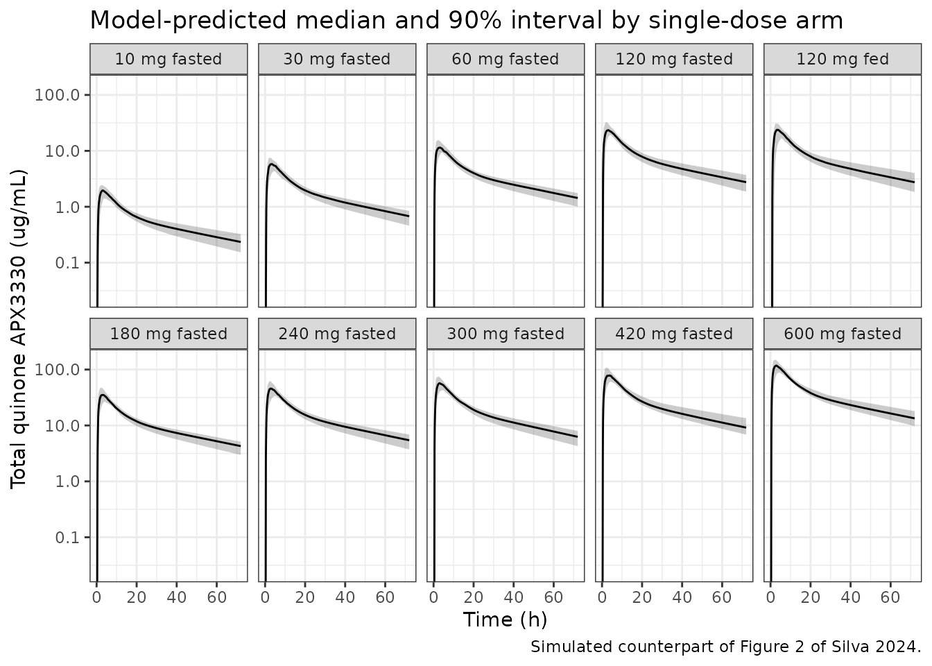

Figure 3 – the food effect on absorption

Silva 2024 Figure 3 plots GastroPlus-predicted dissolution and absorption profiles, which this model cannot produce. What the popPK model does encode is the food effect on the absorption lag time, shown below at 120 mg.

sim |>
  dplyr::filter(dose_mg == 120, time <= 24) |>
  dplyr::group_by(treatment, time) |>
  dplyr::summarise(Q50 = stats::quantile(Cc, 0.50), .groups = "drop") |>
  ggplot(aes(time, Q50, colour = treatment)) +
  geom_line(linewidth = 0.9) +
  labs(
    x = "Time (h)", y = "Total quinone APX3330 (ug/mL)",
    colour = NULL,
    title = "Median predicted 120 mg profile, fasted vs fed",
    caption = "The popPK food effect acts only on the absorption lag time."
  ) +
  theme_bw() +
  theme(legend.position = "bottom")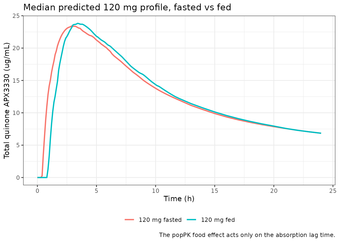

Deterministic structural checks

These use typical-value simulations (omega = NA, sigma = NA) so each result is an exact consequence of the packaged parameters rather than a Monte Carlo estimate. Each is asserted, so the vignette fails to render if the packaged model drifts.

typical_profile <- function(dose, WT, FED, DIS_CANCER, times = obs_times) {
  ev <- rxode2::et(amt = dose, cmt = "depot") |>
    rxode2::et(times, cmt = "central")
  rxode2::rxSolve(
    mod, ev,
    omega = NA, sigma = NA,
    params = c(WT = WT, FED = FED, DIS_CANCER = DIS_CANCER)
  ) |>
    as.data.frame()
}

# Closed-form apparent clearance implied by the packaged parameters.
clf <- function(WT, DIS_CANCER) 0.193 * exp(0.409 * DIS_CANCER) * (WT / 70)^0.659

1. AUC(0-inf) identity

For a linear model, AUC(0-inf) after a single oral dose is exactly dose / (CL/F) regardless of the absorption parameters. This is a free, exact check that CL/F and the weight model are wired correctly.

p120 <- typical_profile(120, WT = 62.4, FED = 0, DIS_CANCER = 0)

# Trapezoidal AUC to 336 h plus the terminal-slope extrapolation.
auc_obs <- sum(diff(p120$time) * (utils::head(p120$Cc, -1) + utils::tail(p120$Cc, -1)) / 2)
tail_fit <- stats::lm(log(Cc) ~ time, data = subset(p120, time >= 168))
lambda_z <- -stats::coef(tail_fit)[["time"]]
auc_inf <- auc_obs + utils::tail(p120$Cc, 1) / lambda_z

auc_expected <- 120 / clf(62.4, 0)
c(simulated = auc_inf, expected = auc_expected,
  ratio = auc_inf / auc_expected)
#>  simulated   expected      ratio 
#> 670.816982 670.682386   1.000201

stopifnot(abs(auc_inf / auc_expected - 1) < 0.001)

2. Dose linearity across 10-600 mg

The paper found neither dose nor period to be a significant covariate, “indicating linear PKs over the range of 10-600 mg oral dosing”. The packaged model must therefore give a dose-normalised exposure that is identical at every dose level.

dose_levels <- c(10, 30, 60, 120, 180, 240, 300, 420, 600)

lin <- vapply(dose_levels, function(d) {
  p <- typical_profile(d, WT = 62.4, FED = 0, DIS_CANCER = 0, times = seq(0, 72, by = 0.1))
  max(p$Cc) / d
}, numeric(1))

data.frame(dose_mg = dose_levels, cmax_per_mg = lin)
#>   dose_mg cmax_per_mg
#> 1      10   0.1994285
#> 2      30   0.1994285
#> 3      60   0.1994285
#> 4     120   0.1994285
#> 5     180   0.1994285
#> 6     240   0.1994285
#> 7     300   0.1994285
#> 8     420   0.1994285
#> 9     600   0.1994285

# Exactly linear: dose-normalised Cmax is identical to numerical precision.
stopifnot(max(abs(lin / lin[1] - 1)) < 1e-8)

3. Oncology-cohort clearance contrast

# The DIS_CANCER effect is a pure log-additive shift on CL/F, so the exposure
# ratio at equal body weight is exactly exp(-0.409).
ratio_at_equal_wt <- clf(70, 0) / clf(70, 1)
c(exposure_ratio_cancer_vs_hv = ratio_at_equal_wt,
  clf_increase_pct = 100 * (exp(0.409) - 1))
#> exposure_ratio_cancer_vs_hv            clf_increase_pct 
#>                   0.6643142                  50.5311720

stopifnot(abs(ratio_at_equal_wt - exp(-0.409)) < 1e-12)

# At the cohorts' actual mean weights the weight effect adds to the disease
# effect: 88.3 kg patients vs 62.4 kg volunteers.
c(clf_hv_62.4kg_mL_per_h = 1000 * clf(62.4, 0),
  clf_cancer_88.3kg_mL_per_h = 1000 * clf(88.3, 1))
#>     clf_hv_62.4kg_mL_per_h clf_cancer_88.3kg_mL_per_h 
#>                   178.9222                   338.5729

4. Food effect: a pure time shift

Because food acts only on t_lag, the packaged model predicts that food shifts the whole profile later by exactly 0.401 * (exp(0.815) - 1) hours and leaves Cmax and AUC untouched.

shift_expected <- 0.401 * (exp(0.815) - 1)
tt <- seq(0, 72, by = 0.01)

fasted <- typical_profile(120, 62.4, FED = 0, DIS_CANCER = 0, times = tt)
fed <- typical_profile(120, 62.4, FED = 1, DIS_CANCER = 0, times = tt)
# The same fed profile, sampled on a grid translated forward by the expected
# shift. If food is a pure time shift, this must lie on top of the fasted
# profile point for point.
fed_shifted <- typical_profile(120, 62.4, FED = 1, DIS_CANCER = 0,
                               times = tt + shift_expected)

tmax_fasted <- fasted$time[which.max(fasted$Cc)]
tmax_fed <- fed$time[which.max(fed$Cc)]

c(tmax_fasted = tmax_fasted, tmax_fed = tmax_fed,
  shift_observed = tmax_fed - tmax_fasted, shift_expected = shift_expected)
#>    tmax_fasted       tmax_fed shift_observed shift_expected 
#>      3.0300000      3.5400000      0.5100000      0.5049294

stopifnot(abs((tmax_fed - tmax_fasted) - shift_expected) < 0.02)

# Pure translation: after removing the shift, the two profiles agree to solver
# tolerance everywhere past the absorption lag. This also establishes that the
# extent of absorption is unchanged, matching "the extent of absorption remains
# the same with or without food co-administration" (Discussion).
post_lag <- fasted$time > 1
rel_diff <- abs(fed_shifted$Cc[post_lag] - fasted$Cc[post_lag]) / fasted$Cc[post_lag]
c(max_relative_difference = max(rel_diff),
  cmax_ratio = max(fed_shifted$Cc) / max(fasted$Cc))
#> max_relative_difference              cmax_ratio 
#>            1.433488e-14            1.000000e+00

stopifnot(max(rel_diff) < 1e-4)
stopifnot(abs(max(fed_shifted$Cc) / max(fasted$Cc) - 1) < 1e-6)

PKNCA validation

sim_nca <- sim |>
  dplyr::filter(!is.na(Cc)) |>
  dplyr::select(id, time, Cc, treatment)

# Guarantee a time-zero record per subject; pre-dose concentration after an
# extravascular dose is 0.
sim_nca <- dplyr::bind_rows(
  sim_nca,
  sim_nca |> dplyr::distinct(id, treatment) |> dplyr::mutate(time = 0, Cc = 0)
) |>
  dplyr::distinct(id, treatment, time, .keep_all = TRUE) |>
  dplyr::arrange(id, treatment, time)

conc_obj <- PKNCA::PKNCAconc(sim_nca, Cc ~ time | treatment + id)

dose_df <- events |>
  dplyr::filter(evid == 1) |>
  dplyr::select(id, time, amt, treatment)

dose_obj <- PKNCA::PKNCAdose(dose_df, amt ~ time | treatment + id)

intervals <- data.frame(
  start = 0, end = Inf,
  cmax = TRUE, tmax = TRUE, aucinf.obs = TRUE, half.life = TRUE
)

nca_res <- PKNCA::pk.nca(PKNCA::PKNCAdata(conc_obj, dose_obj, intervals = intervals))

Comparison against the published NCA

Silva 2024 Table 3 reports observed AUC(0-inf), Cmax and Tmax for each dose arm. Those observed values were the reference against which the GastroPlus model was scored, but they are summaries of the same underlying clinical data the popPK model was fitted to, so they are a legitimate external check on the packaged model.

published <- tibble::tribble(
  ~treatment,       ~cmax, ~tmax, ~aucinf.obs,
  "10 mg fasted",    2.08,   2.0,        52.2,
  "30 mg fasted",    6.41,   3.0,       166.0,
  "60 mg fasted",   13.10,   2.0,       333.0,
  "120 mg fasted",  28.00,   2.0,       690.0,
  "120 mg fed",     24.50,   6.0,       753.0,
  "180 mg fasted",  34.70,   3.0,       987.0,
  "240 mg fasted",  46.90,   3.0,      1281.0,
  "300 mg fasted",  60.20,   3.0,      1839.0,
  "420 mg fasted",  90.80,   3.0,      2728.0,
  "600 mg fasted", 124.00,   2.0,      3588.0
)

cmp <- nlmixr2lib::ncaComparisonTable(
  simulated = nca_res,
  reference = published,
  by = "treatment",
  params = c("cmax", "tmax", "aucinf.obs"),
  units = c(cmax = "ug/mL", tmax = "h", aucinf.obs = "ug*h/mL"),
  tolerance_pct = 20
)

knitr::kable(
  cmp,
  digits = 2,
  caption = paste(
    "Simulated (median of the virtual healthy-volunteer cohort, individual",
    "predictions) vs observed values in Silva 2024 Table 3.",
    "* marks a difference greater than 20%."
  )
)

Simulated (median of the virtual healthy-volunteer cohort, individual predictions) vs observed values in Silva 2024 Table 3. * marks a difference greater than 20%.

NCA parameter	treatment	Reference	Simulated	% diff
Cmax (ug/mL)	10 mg fasted	2.08	1.96	-5.9%
Cmax (ug/mL)	30 mg fasted	6.41	5.97	-6.9%
Cmax (ug/mL)	60 mg fasted	13.1	11.6	-11.1%
Cmax (ug/mL)	120 mg fasted	28	24	-14.2%
Cmax (ug/mL)	120 mg fed	24.5	24	-2.2%
Cmax (ug/mL)	180 mg fasted	34.7	35.6	+2.7%
Cmax (ug/mL)	240 mg fasted	46.9	46.7	-0.5%
Cmax (ug/mL)	300 mg fasted	60.2	57.3	-4.8%
Cmax (ug/mL)	420 mg fasted	90.8	79.7	-12.3%
Cmax (ug/mL)	600 mg fasted	124	119	-4.1%
Tmax (h)	10 mg fasted	2	3.2	+60.0%*
Tmax (h)	30 mg fasted	3	3.3	+10.0%
Tmax (h)	60 mg fasted	2	2.95	+47.5%*
Tmax (h)	120 mg fasted	2	2.8	+40.0%*
Tmax (h)	120 mg fed	6	3.4	-43.3%*
Tmax (h)	180 mg fasted	3	2.9	-3.3%
Tmax (h)	240 mg fasted	3	2.95	-1.7%
Tmax (h)	300 mg fasted	3	3.05	+1.7%
Tmax (h)	420 mg fasted	3	3.35	+11.7%
Tmax (h)	600 mg fasted	2	2.9	+45.0%*
AUC0-∞ (obs) (ug*h/mL)	10 mg fasted	52.2	56.9	+9.1%
AUC0-∞ (obs) (ug*h/mL)	30 mg fasted	166	169	+1.7%
AUC0-∞ (obs) (ug*h/mL)	60 mg fasted	333	351	+5.3%
AUC0-∞ (obs) (ug*h/mL)	120 mg fasted	690	680	-1.5%
AUC0-∞ (obs) (ug*h/mL)	120 mg fed	753	676	-10.2%
AUC0-∞ (obs) (ug*h/mL)	180 mg fasted	987	1020	+3.3%
AUC0-∞ (obs) (ug*h/mL)	240 mg fasted	1280	1360	+5.8%
AUC0-∞ (obs) (ug*h/mL)	300 mg fasted	1840	1600	-12.8%
AUC0-∞ (obs) (ug*h/mL)	420 mg fasted	2730	2290	-16.0%
AUC0-∞ (obs) (ug*h/mL)	600 mg fasted	3590	3260	-9.1%

Reading the comparison

AUC(0-inf) and Cmax reproduce the published values across the whole 10-600 mg range: every one of the twenty rows is within the 20% tolerance. Cmax spans -14.2% to +2.7% and AUC(0-inf) spans -16.0% to +9.1%, with no systematic trend in dose. This is the substantive result – a single set of parameters recovers both the magnitude and the dose-proportionality of the observed exposure over a 60-fold dose range. Note that the packaged model was fitted to the pooled concentration data, whereas the Table 3 observed values are arm-level NCA summaries, so exact agreement is not expected.

Every starred row is a Tmax row, and they have two distinct causes.

The fed arm (-43.3%) is the model’s known structural weak point. The observed Tmax moves from 2 h fasted to 6 h fed, a 4 h shift, but the popPK food effect acts only on t_lag and can therefore shift the profile by only 0.401 * (exp(0.815) - 1) = 0.50 h. This shortfall is not an extraction error; it is precisely the gap that motivated the paper’s second model. Food also affected ka during forward inclusion but “did not meet the inclusion criteria on backward elimination, and hence is not included as a covariate effect in the final model”, so the final popPK model has no mechanism for a larger delay. The authors turned to the GastroPlus ACAT model to explain the observed shift, and that model predicted Tmax moving from 2 h to 5.5 h. Do not tune e_fed_tlag to close this gap – the gap is a faithful property of the published popPK model.

The four starred fasted arms (10, 60, 120 and 600 mg) are an artefact of comparing a continuous prediction against a nominal sampling grid. Every one of the nine published fasted Tmax values is exactly 2.0 or 3.0 h, which is the signature of a Tmax read off the highest nominal sampling time rather than estimated. The model’s fasted Tmax is 2.8-3.35 h in every arm, i.e. it sits between those two grid points and rounds to 3 h. Where the published value happens to be 3.0 h the agreement looks excellent (-3.3% to +11.7%); where it happens to be 2.0 h the same prediction is flagged at +40% to +60%. The underlying prediction is identical across all nine arms – the model has no dose dependence in absorption – so the star pattern reflects the reference’s quantisation, not model error. A percentage tolerance is also unusually harsh on a 2 h quantity: the largest starred discrepancy, 10 mg fasted, is 1.2 h in absolute terms.

Residual-error scale

The comparison above uses Cc (the individual prediction). The observed values in Table 3 are NCA summaries of assayed concentrations, which carry the 16% proportional residual error. Cmax is the one metric biased upward by that noise, because it is an extremum: the more samples a profile has, the more chances the noise gets to produce a high one.

scale_cmp <- sim |>
  dplyr::filter(!is.na(Cc)) |>
  dplyr::group_by(treatment, id) |>
  dplyr::summarise(
    cmax_ipred = max(Cc),
    cmax_obs_scale = max(sim),
    .groups = "drop"
  ) |>
  dplyr::group_by(treatment) |>
  dplyr::summarise(
    `Cmax, IPRED (ug/mL)` = stats::median(cmax_ipred),
    `Cmax, with residual error (ug/mL)` = stats::median(cmax_obs_scale),
    `Inflation (%)` = 100 * (stats::median(cmax_obs_scale) / stats::median(cmax_ipred) - 1),
    .groups = "drop"
  ) |>
  dplyr::mutate(treatment = factor(treatment, levels = arms$treatment)) |>
  dplyr::arrange(treatment) |>
  dplyr::rename("Arm" = treatment)

knitr::kable(scale_cmp, digits = 2,
             caption = "Effect of the 16% proportional residual error on median Cmax.")

Effect of the 16% proportional residual error on median Cmax.

Arm	Cmax, IPRED (ug/mL)	Cmax, with residual error (ug/mL)	Inflation (%)
10 mg fasted	1.96	2.55	30.18
30 mg fasted	5.97	7.52	25.92
60 mg fasted	11.64	15.72	35.03
120 mg fasted	24.02	31.16	29.70
120 mg fed	23.95	30.69	28.10
180 mg fasted	35.63	47.37	32.95
240 mg fasted	46.67	58.59	25.53
300 mg fasted	57.31	73.29	27.89
420 mg fasted	79.67	103.20	29.54
600 mg fasted	118.89	153.91	29.46

The inflation is about 30% here, which is not a usable estimate of the bias in the published numbers – it is an artefact of this vignette’s sampling grid. Each simulated profile carries 253 observations, so the observed-scale Cmax is the maximum of 253 noisy draws and is pushed far into the upper tail. The real studies sampled on the order of ten to fifteen times per profile, where the same 16% residual error produces a much smaller upward bias. This is exactly why the comparison table above is built on Cc rather than on sim: the IPRED scale is free of a bias that depends on a design choice made in this vignette rather than on the model. It is, however, the right direction to explain why the observed Cmax values sit modestly above the IPRED predictions in eight of the ten arms.

Assumptions and deviations

• Only the population PK model is packaged. The paper’s companion semi-mechanistic absorption model is a GastroPlus 9.8 ACAT model. Its gastrointestinal compartment structure, transit times, volumes and pH profile are platform-internal, its fasted/fed physiology set is in Table S5 (not in the open-access deposit), and its dissolution model has no rxode2 analogue. The paper does report the tuned absorption scale factors and the C1-C4 coefficients (Table 1), but those are inputs to a structure that is not published, so the model cannot be reconstructed. Note also that the two-compartment disposition block used inside GastroPlus (Table 1: CL 0.183 L/h, central volume 3 L, k12 0.11158/h, k21 0.0669/h) is a separate parameterisation from the popPK model’s apparent values and is not the same model.

• The omega and gamma entries in Table 2 are read as standard deviations, per Monolix convention, and squared to give the ini() variances. Two independent statements in the paper’s own text confirm the reading (see “Reading the Monolix variance parameters” above).

• Inter-occasion variability is not carried as occasion-indexed etas. Table 2 reports IOV on t_lag (gamma 0.515) and ka (gamma 0.564) alongside IIV on ka, CL/F and V1/F. This file applies the established nlmixr2lib convention for between-occasion variability (Svensson_2012_nevirapine.R, Bienczak_2016_nevirapine.R, Bukkems_2021_raltegravir.R): drop the occasion term when a between-subject term is reported on the same parameter, and fold it in as a between-subject-equivalent when only the occasion term is reported. So ka keeps omega = 0.517 and drops gamma = 0.564, while t_lag – which has no IIV row at all – takes etaltlag ~ 0.515^2. The occasion-indicator encoding used in Chen_2023_nemonoxacin.R is not available here because Silva 2024 never states how many occasions the IOV spans: the dose-escalation arm gave three single-dose occasions per subject and the food-effect crossover gave two. Encoding IOV explicitly would require inventing that occasion count. Consequence for simulation: total ka variability within a subject is understated relative to the published model (an SD of 0.517 rather than sqrt(0.517^2 + 0.564^2) = 0.765).

• The t_lag ~ ka correlation of -0.476 is not encoded. Table 2 groups it under “Correlations” with the CL/F-V1/F correlation, but t_lag has no omega row, so this correlation is necessarily between the two IOV terms (gamma_tlag and gamma_ka), not between IIV terms. Because gamma_ka is dropped and etaltlag is a folded gamma_tlag, pairing -0.476 with the IIV etalka would mix variability levels. The two etas are left independent. The CL/F-V1/F correlation of 0.349, which is an IIV-level correlation, is encoded as a block.

• The categorical covariate effects follow the paper’s printed Equation 2, not its percentage claims. Equation 2 is p_j = p_pop x exp(beta_cov x cov_j), which is also Monolix’s standard parameterisation for a categorical covariate on a log-normally distributed parameter. Under that equation beta_SubjectSource,CL = 0.409 means CL/F is exp(0.409) - 1 = 50.5% higher in patients with cancer, and beta_Food,tlag = 0.815 means the lag time is exp(0.815) - 1 = 126% higher when dosed fed. The paper’s text instead reports “41%” and “80-81%”, which are beta read directly as a fraction (0.409 -> 40.9%, 0.815 -> 81.5%) – the same slip made consistently for both coefficients, in the abstract, Results and Discussion. Since the printed equation and the estimation software agree with each other, and nothing in the data discriminates (the fed-state Tmax shift is 0.50 h under the exponential reading and 0.33 h under the linear one, against a 4 h observed shift, so both readings miss it), the equation is used. A user who wants the literal-percentage reading can set e_cancer_cl <- log(1.409) and e_fed_tlag <- log(1.815).

• Body weight is treated as time-fixed. Weights were measured on three to eight occasions in the oncology cohort, but the paper states there was “no trend in weight over the course of the study”.

• Serum albumin is documented but not modelled. It is recorded in the model file’s covariatesDataExcluded list. The paper screened it, found it significant on its own (delta -2LL = -25.1), and deliberately replaced it with the DIS_CANCER subject-source indicator, which gave a larger drop (delta -2LL = -39.52) and absorbs the other between-cohort differences. No usable albumin coefficient is reported.

• The virtual cohort’s weight distribution is constructed, not published. Weights are a deterministic quantile grid of a normal distribution with the reported mean (62.4 kg) and an SD of 5.6 kg chosen so that the reported 52-77 kg range spans roughly the full grid; values are clipped to that range. The paper reports only the mean and range (Table S3 holds the full demographics and is not in the open-access deposit).

• The oncology cohort is exercised only through typical-value calculations. The paper reports a mean weight of 88.3 kg for those 19 patients but no spread, so a virtual oncology cohort would require inventing a weight distribution. The clearance contrast is instead verified in closed form.

• The two multiple-dose rows of Table 3 are not reproduced. The “120 mg q.d., fed” and “120 mg b.i.d., fed” rows report AUC over a steady-state dosing interval (168-180 h for b.i.d. or 192 h for q.d. per the table footnote), not AUC(0-inf), so they are not comparable to the single-dose interval used above.

• Unit conversion. The paper reports clearances in mL/h and volumes in mL. The packaged model uses L and L/h so that a dose in mg over a volume in L yields mg/L, which equals the ug/mL used in the paper’s Table 3. Every conversion is a factor of 1000 and is noted on the relevant parameter line in the model file.