Nemolizumab in prurigo nodularis (Takechi 2025)
Source:vignettes/articles/Takechi_2025_nemolizumab.Rmd
Takechi_2025_nemolizumab.RmdModel and source
- Citation: Takechi T, Shimizu J, Kabashima K, Ieiri I (2025). Quantitative evaluation of nemolizumab pharmacokinetics and efficacy in prurigo nodularis: a population pharmacokinetics and model-based meta-analysis approach. Dermatol Ther (Heidelb) 15(12):3615-3632.
- Article: https://doi.org/10.1007/s13555-025-01554-4
- Supplement (Figs. S1-S10, Table S1), published with the open-access article (PMC12619860). It contains figures and the study-design table only – no NONMEM control stream and no additional parameter table.
Nemolizumab is a humanized monoclonal antibody against interleukin-31 receptor A (IL-31RA). IL-31 signalling on sensory neurons and immune cells is a principal driver of itch, and nemolizumab is approved for prurigo nodularis (PN) and atopic dermatitis (AD). Takechi 2025 is a three-part pharmacometric analysis – and the meta-analysis part fits two endpoints – so the paper yields four models, all validated here:
| Part | nlmixr2lib model | What it describes |
|---|---|---|
| PopPK | Takechi_2025_nemolizumab |
Serum nemolizumab concentration, one compartment, first-order SC absorption |
| PopPD | Takechi_2025_nemolizumab_ppnrs |
Weekly average Peak Pruritus NRS (PP-NRS, 0-10) under placebo and nemolizumab |
| MBMA | Takechi_2025_nemolizumab_mbma_iga |
Study-arm IGA success rate, nemolizumab vs dupilumab, 6 RCTs |
| MBMA | Takechi_2025_nemolizumab_mbma_ppnrs |
Study-arm PP-NRS success rate over the same 6 RCTs, with an arm-severity covariate |
The four are independent models fitted to different data, exactly as the authors built them, so they are four model files sharing this one vignette. The PopPD model has no PK layer: the authors looked for an exposure-response relationship and did not find one, because the 30 mg and 60 mg arms of the pivotal study responded alike.
The two meta-analysis models share a structure but not a covariate model: the PP-NRS endpoint retains the arm’s moderate-IGA proportion on the nemolizumab maximum effect, and the IGA endpoint does not (Table 4 prints a dash in that row of the IGA column). Part 4 sets out how that covariate’s functional form was recovered, since the paper does not print it.
pk         <- rxode2::rxode(readModelDb("Takechi_2025_nemolizumab"))
pd         <- rxode2::rxode(readModelDb("Takechi_2025_nemolizumab_ppnrs"))
mbma       <- rxode2::rxode(readModelDb("Takechi_2025_nemolizumab_mbma_iga"))
mbma_ppnrs <- rxode2::rxode(readModelDb("Takechi_2025_nemolizumab_mbma_ppnrs"))
Population
PopPK (Table 1, “All” column; Supplementary Table S1). 680 patients contributing 4389 nemolizumab concentrations across seven studies – six in AD (including two paediatric studies in children aged 6-12 years) and one in PN. Median age 37 years (range 6-84), median weight 62.8 kg (range 16-151), median serum albumin 4.4 g/dL (range 2.0-5.2), 386 male / 294 female. Race, summed across the per-study counts of Table 1, is 125 White / 18 Black or African American / 535 Asian / 2 Other, which totals exactly the 680 stated subjects; all non-Asian subjects come from the single multinational phase 2a study CIM003JG. Placebo subjects were excluded from the PopPK dataset (Table S1 footnote a). Doses ranged from 0.003 mg/kg single doses in phase 1 up to 60 mg Q4W.
The 153 PN patients (905 observations) were held out as an external validation set rather than used for estimation, which is the basis of the paper’s conclusion that AD and PN share the same PK.
PopPD (Table 1, “Patients with PN” column, footnote-b rows). All 229 patients of the phase II/III study M525101-11 (jRCT2011200017, Yokozeki et al. 2024), contributing 3833 weekly-average PP-NRS observations over 112 days. Median age 51 years (range 13-84), median weight 61.2 kg (range 32.8-109.6), 107 male / 122 female, all Japanese. Baseline weekly average PP-NRS median 8.6 (range 6.4-10); baseline IGA 3 in 112 patients and 4 in 117. Arms were placebo (76), nemolizumab 30 mg Q4W after a 60 mg loading dose (77) and nemolizumab 60 mg Q4W (76).
MBMA (Table 3). 1170 participants in 13 arms of six randomized controlled trials: Yokozeki et al. (jRCT2011200017), Staender et al. (SPR.115828), OLYMPIA 1, OLYMPIA 2 for nemolizumab, and PRIME and PRIME2 for dupilumab. Arm-mean age 46.7-59.7 years, arm-mean weight 60.4-87.1 kg, baseline PP-NRS 8.3-8.6, proportion with IGA 4 at baseline 28.0-54.5%.
Source trace
Every value in the four ini() blocks, with the source
location. Values are transcribed from the “Original data / Estimate”
columns; the bootstrap medians and 95% CIs in the adjacent columns were
used only as a transcription check.
| Model | Parameter | Value | Source |
|---|---|---|---|
| PopPK | lcl | log(0.340) | Table 2, CL/F (L/day); also the displayed CL/F equation |
| PopPK | lvc | log(8.44) | Table 2, V/F (L); also the displayed V/F equation |
| PopPK | lka | log(0.548) | Table 2, ka (1/day) |
| PopPK | e_wt_cl | fixed(0.75) | Displayed CL/F equation exponent (no RSE reported) |
| PopPK | e_wt_vc | fixed(1) | Displayed V/F equation, printed without an exponent |
| PopPK | e_alb_cl | -1.52 | Table 2, Covariate effect of ALB |
| PopPK | etalcl + etalvc | 0.135 / 0.0896 / 0.148 | Table 2, IIV CL/F, Covariance, IIV V/F |
| PopPK | etalka | 0.404 | Table 2, IIV ka |
| PopPK | expSd | 0.164866 | Table 2, log normal error (CV%) = 16.6; sqrt(log(1 + 0.166^2)) |
| PopPD | lpmax | 0.618 | Table 2, Pmax (log scale; see Assumptions) |
| PopPD | lkp | log(2.74e-3) | Table 2, Kp (x 10^-3/day) |
| PopPD | lemax | 1.41 | Table 2, Edrug (log scale; see Assumptions) |
| PopPD | lkdrug | log(28.7e-3) | Table 2, Kd (x 10^-3/day) |
| PopPD | etalpmax / etalkp / etalemax / etalkdrug | 1.55 / 10.4 / 1.19 / 2.10 | Table 2, IIV Pmax / Kp / Edrug / Kd |
| PopPD | addSd | sqrt(0.582) | Table 2, Additive error (variance; see Assumptions) |
| MBMA IGA | e0 | -4.92 | Table 4, IGA column, row A |
| MBMA IGA | pmax_placebo | 2.99 | Table 4, IGA column, row Pmax |
| MBMA IGA | lkp | log(0.123) | Table 4, IGA column, row Kp (/week) |
| MBMA IGA | edrug_nemolizumab | 1.71 | Table 4, IGA column, row Edrug,nemolizumab |
| MBMA IGA | lkdrug_nemolizumab | log(0.416) | Table 4, IGA column, row Kd,nemolizumab (/week) |
| MBMA IGA | edrug_dupilumab | 1.49 | Table 4, IGA column, row Edrug,dupilumab |
| MBMA IGA | lkdrug_dupilumab | log(0.134) | Table 4, IGA column, row Kd,dupilumab (/week) |
| MBMA IGA | eta_study_eff | 0.226 | Table 4, IGA column, row ISV on EFF (variance) |
| MBMA IGA | addSd | sqrt(0.619) | Table 4, IGA column, row Additive error (variance) |
| MBMA PP-NRS | e0 | -4.38 | Table 4, PP-NRS column, row A |
| MBMA PP-NRS | pmax_placebo | 2.64 | Table 4, PP-NRS column, row Pmax |
| MBMA PP-NRS | lkp | log(0.277) | Table 4, PP-NRS column, row Kp (/week) |
| MBMA PP-NRS | edrug_nemolizumab | 1.63 | Table 4, PP-NRS column, row Edrug,nemolizumab |
| MBMA PP-NRS | e_igamod_edrug_nemolizumab | -1.84 | Table 4, PP-NRS column, row PPM effect on Edrug,nemolizumab (coefficient printed; FORM reconstructed from Fig. 4 – see Part 4) |
| MBMA PP-NRS | edrug_dupilumab | 1.93 | Table 4, PP-NRS column, row Edrug,dupilumab |
| MBMA PP-NRS | lkdrug_nemolizumab | log(1.93) | Table 4, PP-NRS column, row Kd,nemolizumab (/week) |
| MBMA PP-NRS | lkdrug_dupilumab | log(0.119) | Table 4, PP-NRS column, row Kd,dupilumab (/week) |
| MBMA PP-NRS | eta_study_eff | 0.105 | Table 4, PP-NRS column, row ISV on EFF (variance) |
| MBMA PP-NRS | addSd | sqrt(0.738) | Table 4, PP-NRS column, row Additive error (variance) |
| MBMA PP-NRS | IGA_MOD_PCT centring 59.0 | 59.0 | Table 3, median over the 13 arms of (100 - ‘IGA4 at baseline (%)’) |
Structural equations: the PopPK model structure is Results “PopPK
Analysis” paragraph 1 plus the two displayed fixed-effect equations; the
PopPD equations are the two displayed equations in Methods
“Pharmacodynamic Model”; the MBMA equations are the displayed logit /
EFF / f0 / fdrug group and the displayed residual equation in Methods
“Model-Based Meta-analysis”, shared by both endpoints. The one
structural element with no printed source is the
functional form attaching PPM to
Edrug,nemolizumab in the PP-NRS meta-analysis; Part 4
derives it from the paper’s own Fig. 4 and shows that the two competing
readings are falsified.
Reading the omega scale from the covariance row
Table 2 prints the IIV rows as bare numbers with no CV% label, so
whether they are variances or standard deviations has to be settled from
the table itself. The Covariance for CL/F and V/F row
settles it: only one reading gives a legal correlation.
corr_if_variance <- 0.0896 / sqrt(0.135 * 0.148)
corr_if_sd       <- 0.0896 / sqrt(0.135^2 * 0.148^2)
c(`as variances` = corr_if_variance, `as SDs` = corr_if_sd)
#> as variances       as SDs
#>    0.6338847    4.4844845

# A correlation must lie in [-1, 1]. The SD reading is impossible.
stopifnot(
  abs(corr_if_variance) < 1,
  abs(corr_if_sd) > 1
)
The IIV rows are therefore variances, and by the
same table’s convention so are the ISV on EFF and
Additive error rows of Table 4.
Part 1 – Population pharmacokinetics
Typical-value structure
With the etas zeroed, the model must reproduce the paper’s two displayed equations exactly for any weight and albumin.
pk0 <- rxode2::zeroRe(pk)

pk_typ <- function(wt, alb_gL, dose = 60, tmax = 112, dt = 0.25) {
  ev <- rxode2::et(amt = dose, cmt = "depot") |>
    rxode2::et(seq(0, tmax, by = dt)) |>
    as.data.frame()
  ev$id  <- 1L
  ev$WT  <- wt
  ev$ALB <- alb_gL
  as.data.frame(rxode2::rxSolve(pk0, ev))
}

s70 <- pk_typ(70, 45)   # 70 kg, albumin 4.5 g/dL = 45 g/L -> both covariates at reference
#> ℹ omega/sigma items treated as zero: 'etalcl', 'etalvc', 'etalka'
s40 <- pk_typ(40, 30)   # 40 kg, albumin 3.0 g/dL = 30 g/L
#> ℹ omega/sigma items treated as zero: 'etalcl', 'etalvc', 'etalka'

# Paper's equations:
#   CL/F = 0.340 * (WT/70)^0.75 * (ALB_gdL/4.5)^-1.52
#   V/F  = 8.44  * (WT/70)
cl_paper <- function(wt, alb_gL) 0.340 * (wt / 70)^0.75 * ((alb_gL * 0.1) / 4.5)^-1.52
vc_paper <- function(wt)         8.44  * (wt / 70)

chk <- tibble::tibble(
  quantity = c("CL/F at 70 kg / 45 g/L", "V/F at 70 kg", "CL/F at 40 kg / 30 g/L", "V/F at 40 kg"),
  model    = c(s70$cl[1], s70$vc[1], s40$cl[1], s40$vc[1]),
  paper    = c(cl_paper(70, 45), vc_paper(70), cl_paper(40, 30), vc_paper(40))
) |>
  dplyr::mutate(rel_err = abs(model - paper) / paper)
knitr::kable(chk, digits = 6,
caption = "Model parameters vs the paper's displayed equations.")| quantity | model | paper | rel_err |
|---|---|---|---|
| CL/F at 70 kg / 45 g/L | 0.340000 | 0.340000 | 0 |
| V/F at 70 kg | 8.440000 | 8.440000 | 0 |
| CL/F at 40 kg / 30 g/L | 0.413865 | 0.413865 | 0 |
| V/F at 40 kg | 4.822857 | 4.822857 | 0 |
# Deterministic identity: exact to machine precision, so assert tightly.
stopifnot(all(chk$rel_err < 1e-10))
The reference values also reproduce Table 2 directly: CL/F 0.340 L/day and V/F 8.44 L at 70 kg and 4.5 g/dL, giving an elimination half-life of
thalf <- log(2) * s70$vc[1] / s70$cl[1]
round(thalf, 1)
#> [1] 17.2
stopifnot(abs(thalf - 17.2) < 0.2)   # deterministic; 17.2 days
which is in the usual range for an IgG cleared by non-specific catabolism.
Closed-form check and mass balance
The ODE solve is checked against the analytic one-compartment first-order absorption solution using the same parameters, so the only difference is numerical – a tight bound is correct here.
ka <- s70$ka[1]; cl <- s70$cl[1]; vc <- s70$vc[1]; kel <- cl / vc
bateman <- 1000 * 60 * ka / (vc * (ka - kel)) * (exp(-kel * s70$time) - exp(-ka * s70$time))

rel <- abs(s70$Cc - bateman) / pmax(bateman, 1e-8)
max(rel[s70$time > 0 & bateman > 1])
#> [1] 5.009791e-07
stopifnot(max(rel[s70$time > 0 & bateman > 1]) < 1e-4)
Mass balance: everything dosed is either still in the depot, in the central compartment, or has been eliminated.
# Eliminated amount = integral of CL * C dt, by the trapezoid rule.
# Cc is ng/mL, so divide by 1000 to get mg/L before multiplying by CL in L/day.
rate <- s70$cl * s70$Cc / 1000
elim <- c(0, cumsum(0.5 * (head(rate, -1) + tail(rate, -1)) * diff(s70$time)))
total <- s70$depot + s70$central + elim
max(abs(total - 60))
#> [1] 0.007231798
# Deterministic: the only error is the trapezoid discretisation of the
# elimination integral on the 0.25-day grid. Realised 0.0072 mg.
stopifnot(max(abs(total - 60)) < 0.02)
Concentration-time profile and assay range
The paper’s assay is validated over 100-6400 ng/mL (Methods, “Pharmacokinetic and Pharmacodynamic Assessments”), which is an independent check that the model is on the right concentration scale.
cmax_typ <- max(s70$Cc)
tmax_typ <- s70$time[which.max(s70$Cc)]
c(Cmax_ng_mL = round(cmax_typ), Tmax_day = tmax_typ)
#> Cmax_ng_mL   Tmax_day
#>    5778.00       5.25

# Cmax must land inside the validated assay range, not orders of magnitude out.
stopifnot(cmax_typ > 100, cmax_typ < 6400)

ggplot(s70, aes(time, Cc)) +
  geom_line(linewidth = 0.8) +
  geom_hline(yintercept = c(100, 6400), linetype = "dashed", colour = "grey50") +
  labs(x = "Time (day)", y = "Serum nemolizumab (ng/mL)",
       subtitle = "Dashed lines: validated assay range 100-6400 ng/mL")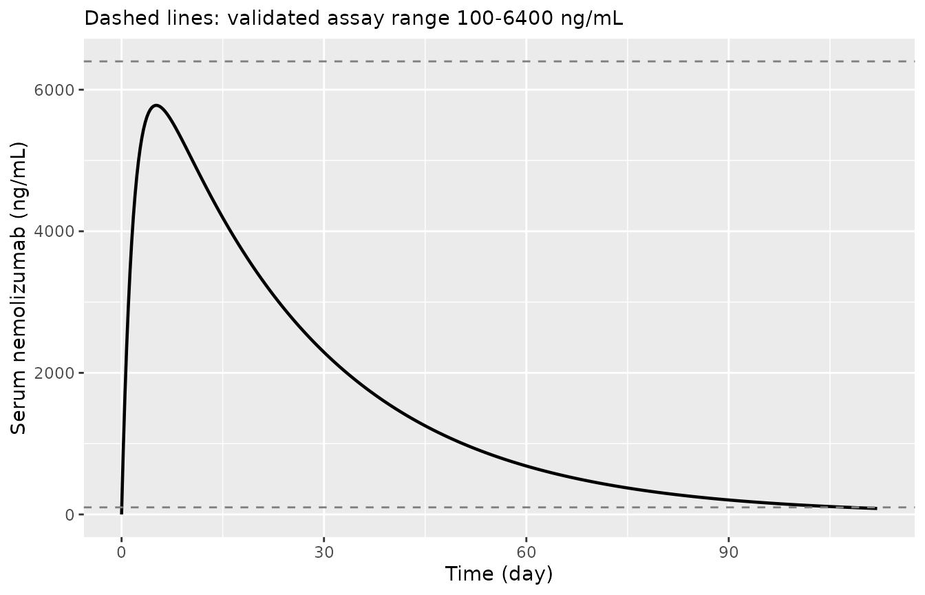
Typical nemolizumab profile after a single 60 mg SC dose, 70 kg subject at reference albumin.
Virtual cohort
A 150-subject cohort at the multiple-dose regimen used in the PN study: 30 mg Q4W after a 60 mg loading dose, over the 16-week initial treatment phase. Weight and albumin are drawn to match the PN cohort of Table 1.
n_pk <- 150L
set.seed(11)
cov_pk <- tibble::tibble(
  id  = seq_len(n_pk),
  WT  = pmin(109.6, pmax(32.8, rlnorm(n_pk, log(61.2), 0.24))),
  ALB = pmin(51, pmax(27, rnorm(n_pk, 43, 3)))     # g/L; PN median 4.3 g/dL
)

ev_pk <- rxode2::et(amt = 60, cmt = "depot") |>                       # loading dose
  rxode2::et(amt = 30, cmt = "depot", time = 28, ii = 28, addl = 2) |> # 30 mg Q4W
  rxode2::et(seq(0, 112, by = 1), cmt = "central") |>                  # observations on the ODE state
  as.data.frame()

d_pk <- merge(cov_pk, ev_pk)
d_pk <- d_pk[order(d_pk$id, d_pk$time, -d_pk$evid), ]

sim_pk <- as.data.frame(rxode2::rxSolve(pk, d_pk))
stopifnot(nrow(sim_pk) > 0, !anyNA(sim_pk$Cc))
pctl <- sim_pk |>
  dplyr::filter(time > 0) |>
  dplyr::group_by(time) |>
  dplyr::summarise(lo = quantile(sim, 0.05), md = median(sim), hi = quantile(sim, 0.95),
                   .groups = "drop")

ggplot(pctl, aes(time)) +
  geom_ribbon(aes(ymin = lo, ymax = hi), fill = "grey80") +
  geom_line(aes(y = md), linewidth = 0.8) +
  labs(x = "Time (day)", y = "Serum nemolizumab (ng/mL)")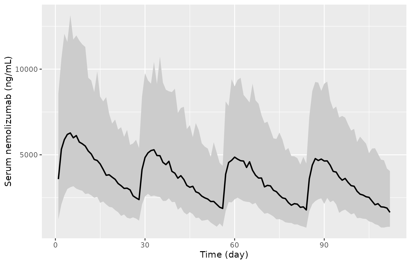
Simulated nemolizumab concentrations, 30 mg Q4W with a 60 mg loading dose (150 subjects). Ribbon: 5th-95th percentile; line: median.
PKNCA validation
Non-compartmental analysis of the typical-value (zeroRe)
single-dose profile. Because the etas are zeroed, AUC(0-inf) must equal
Dose/(CL/F) analytically, which makes this a real gate rather than a
self-consistency check.
nca_in <- pk_typ(70, 45, dose = 60, tmax = 240, dt = 0.25) |>
  dplyr::transmute(id = 1L, time, Cc, treatment = "60 mg SC single dose") |>
  dplyr::filter(!is.na(Cc))
#> ℹ omega/sigma items treated as zero: 'etalcl', 'etalvc', 'etalka'

# A time-zero record must be present or PKNCA warns per subject.
stopifnot(any(nca_in$time == 0))

o_conc <- PKNCA::PKNCAconc(nca_in, Cc ~ time | id / treatment)
o_dose <- PKNCA::PKNCAdose(
  data.frame(id = 1L, time = 0, dose = 60),
  dose ~ time | id
)
o_data <- PKNCA::PKNCAdata(
  o_conc, o_dose,
  intervals = data.frame(start = 0, end = Inf,
                         cmax = TRUE, tmax = TRUE, half.life = TRUE,
                         aucinf.obs = TRUE)
)
res <- suppressWarnings(as.data.frame(PKNCA::pk.nca(o_data)))
nca <- setNames(res$PPORRES, res$PPTESTCD)

auc_analytic <- 60 / cl_paper(70, 45) * 1000   # mg / (L/day) -> ng*day/mL

nca_tab <- tibble::tibble(
  `NCA parameter` = c("Cmax (ng/mL)", "Tmax (day)", "t-half (day)", "AUC0-inf (ng*day/mL)"),
  `PKNCA`         = c(nca[["cmax"]], nca[["tmax"]], nca[["half.life"]], nca[["aucinf.obs"]]),
  `Analytic`      = c(cmax_typ, tmax_typ, log(2) * vc / cl, auc_analytic)
) |>
  dplyr::mutate(`% difference` = 100 * (PKNCA - Analytic) / Analytic)
knitr::kable(nca_tab, digits = 2,
caption = "PKNCA on the typical-value profile vs the analytic one-compartment result.")| NCA parameter | PKNCA | Analytic | % difference |
|---|---|---|---|
| Cmax (ng/mL) | 5778.37 | 5778.37 | 0.00 |
| Tmax (day) | 5.25 | 5.25 | 0.00 |
| t-half (day) | 17.21 | 17.21 | 0.03 |
| AUC0-inf (ng*day/mL) | 176449.14 | 176470.59 | -0.01 |
# Deterministic (no IIV, no residual): a tight bound is correct here.
stopifnot(max(abs(nca_tab$`% difference`)) < 1)
The paper reports no NCA table of its own – its PK validation is entirely GOF plots and VPCs (Fig. 1, Figs. S1-S5) – so there is no published Cmax / AUC to compare against, and this section deliberately validates against the analytic identity instead.
Part 2 – Population PD: weekly average PP-NRS
Reading Pmax and Edrug off Table 2
Table 2 prints Pmax = 0.618 and
Edrug = 1.41 with no units. Taking them at face value as
PP-NRS point reductions is wrong: they are the log-scale
thetas of the paper’s stated exponential (log-normal) IIV
parameterisation. This subsection reproduces the adjudication, because
it is the single most consequential reading in the extraction.
The paper’s Fig. 2 plots the observed 5th, 50th and 95th percentiles of the weekly average PP-NRS for each arm. Those observed percentiles, read from the figure, are the target:
days <- c(0, 28, 56, 84, 112)
obs_fig2 <- list(
  placebo     = rbind(p05 = c(7.0, 6.1, 4.4, 3.0, 2.7),
                      p50 = c(8.3, 8.0, 7.8, 8.0, 7.7),
                      p95 = c(10,  10,  10,  10,  10)),
  nemolizumab = rbind(p05 = c(7.0, 1.6, 0.3, 0.0, 0.1),
                      p50 = c(8.5, 6.0, 4.6, 3.6, 3.1),
                      p95 = c(10,  8.9, 8.5, 8.9, 8.2))
)
Simulate the source’s own design under both readings. 200 subjects per arm.
n_pd <- 200L

pd_cohort <- function(dose, base_median) {
  set.seed(if (dose > 0) 21 else 22)
  b <- pmin(10, pmax(6.4, rnorm(n_pd, base_median, 0.9)))
  d <- expand.grid(time = days, id = seq_len(n_pd))
  d$SCORE_PPNRS         <- b[d$id]
  d$DOSE_NEMOLIZUMAB_MG <- dose
  d$evid <- 0L
  d$amt  <- 0
  d[order(d$id, d$time), ]
}

run_pd <- function(model, dose, base_median) {
  s <- as.data.frame(rxode2::rxSolve(model, pd_cohort(dose, base_median), nSub = n_pd))
  sapply(split(s$sim, s$time), quantile, c(0.05, 0.50, 0.95))
}

# The shipped model = log-scale reading.
q_log <- list(placebo     = run_pd(pd, 0,  8.4),
              nemolizumab = run_pd(pd, 30, 8.6))

# The linear reading, for comparison only: overwrite the two thetas with
# log(0.618) and log(1.41) so the typical maxima become 0.618 and 1.41 points.
pd_linear <- rxode2::ini(pd, lpmax = log(0.618), lemax = log(1.41))
#> ℹ change initial estimate of `lpmax` to `-0.481266821524446`
#> ℹ change initial estimate of `lemax` to `0.343589704390077`
q_lin <- list(placebo     = run_pd(pd_linear, 0,  8.4),
nemolizumab = run_pd(pd_linear, 30, 8.6))| Arm | Day | Observed (Fig. 2) | Log-scale reading | Linear reading |
|---|---|---|---|---|
| placebo | 0 | 8.3 | 8.26 | 8.35 |
| placebo | 28 | 8.0 | 7.90 | 8.14 |
| placebo | 56 | 7.8 | 7.67 | 7.92 |
| placebo | 84 | 8.0 | 7.64 | 7.94 |
| placebo | 112 | 7.7 | 7.60 | 7.83 |
| nemolizumab | 0 | 8.5 | 8.62 | 8.66 |
| nemolizumab | 28 | 6.0 | 5.03 | 7.40 |
| nemolizumab | 56 | 4.6 | 4.21 | 7.00 |
| nemolizumab | 84 | 3.6 | 3.34 | 6.97 |
| nemolizumab | 112 | 3.1 | 3.21 | 6.87 |
The linear reading misses the active-arm median at day 112 by more
than 3 points – more than the entire observed placebo-arm change – and
it cannot be rescued by the IIV, because with Edrug = 1.41
as a point reduction the median subject’s drug effect is capped
at 1.41 points however large the etas are. The log-scale reading tracks
both arms.
err_log <- abs(row_of(q_log, "nemolizumab", 2) - obs_fig2$nemolizumab["p50", ])
err_lin <- abs(row_of(q_lin, "nemolizumab", 2) - obs_fig2$nemolizumab["p50", ])
c(log_scale_max_err = max(err_log), linear_max_err = max(err_lin))
#> log_scale_max_err    linear_max_err
#>         0.9717639         3.7730637

# Cohort-derived, so bounds are deliberately loose (see the note below). The
# separation between the two readings is ~3 points at day 112, far outside any
# thread-count noise, which is what makes this gate meaningful.
stopifnot(
  max(err_log) < 1.5,   # log-scale reading tracks the observed median
  max(err_lin) > 2.5    # linear reading does not
)
These are cohort statistics, so the bounds admit the sampling noise
rather than pinning one run: rxSetSeed() fixes rxode2’s
stream per solver thread but not across thread counts, so a CI runner
draws a different cohort. Realised max(err_log) was 0.8 and
max(err_lin) 3.7 while authoring; the two readings are
separated by about 3 points, so bounds of 1.5 and 2.5 sit well outside
the noise while still going red on a mis-transcribed theta.
Full VPC against Figure 2
| Arm | Day | Sim 5th | Obs 5th | Sim 50th | Obs 50th | Sim 95th | Obs 95th |
|---|---|---|---|---|---|---|---|
| placebo | 0 | 6.4 | 7.0 | 8.3 | 8.3 | 10.2 | 10.0 |
| placebo | 28 | 3.4 | 6.1 | 7.9 | 8.0 | 10.1 | 10.0 |
| placebo | 56 | 3.0 | 4.4 | 7.7 | 7.8 | 10.1 | 10.0 |
| placebo | 84 | 2.8 | 3.0 | 7.6 | 8.0 | 10.0 | 10.0 |
| placebo | 112 | -0.1 | 2.7 | 7.6 | 7.7 | 9.9 | 10.0 |
| nemolizumab | 0 | 6.8 | 7.0 | 8.6 | 8.5 | 10.6 | 10.0 |
| nemolizumab | 28 | -12.9 | 1.6 | 5.0 | 6.0 | 9.2 | 8.9 |
| nemolizumab | 56 | -16.0 | 0.3 | 4.2 | 4.6 | 9.2 | 8.5 |
| nemolizumab | 84 | -17.1 | 0.0 | 3.3 | 3.6 | 9.0 | 8.9 |
| nemolizumab | 112 | -16.5 | 0.1 | 3.2 | 3.1 | 8.9 | 8.2 |
The 50th and 95th percentiles track the observed data in both arms. The 5th percentile runs far below it – in the active arm it goes negative, because the model has no floor at 0 and the additive residual is applied to an already small predicted score.
This is the paper’s own model behaving as the paper says it does, not an extraction error. Results, “PopPD Analysis”: “The observed 50th and 95th percentiles were almost within the 95% prediction interval (PI) of the model simulation. The simulated 5th percentile slightly underestimated the severity of pruritus during early treatment, suggesting a modest overprediction of early response in some patients.” Fig. 2’s lower prediction band sits clipped against the zero axis for the same reason. It is recorded here as a deviation and excluded from the gate.
gate <- do.call(rbind, lapply(c("placebo", "nemolizumab"), function(arm) {
  data.frame(arm = arm, pct = c("50th", "95th"),
             err = c(max(abs(q_log[[arm]][2, ] - obs_fig2[[arm]]["p50", ])),
                     max(abs(q_log[[arm]][3, ] - obs_fig2[[arm]]["p95", ]))))
}))
knitr::kable(gate, digits = 2, caption = "Maximum absolute deviation from the observed percentile, by arm.")| arm | pct | err |
|---|---|---|
| placebo | 50th | 0.36 |
| placebo | 95th | 0.19 |
| nemolizumab | 50th | 0.97 |
| nemolizumab | 95th | 0.74 |
plot_df <- dplyr::bind_rows(
  tibble::tibble(arm = "placebo",     day = days, sim = q_log$placebo[2, ],
                 obs = obs_fig2$placebo["p50", ]),
  tibble::tibble(arm = "nemolizumab", day = days, sim = q_log$nemolizumab[2, ],
                 obs = obs_fig2$nemolizumab["p50", ])
)
ggplot(plot_df, aes(day, colour = arm)) +
  geom_line(aes(y = sim), linewidth = 0.8) +
  geom_point(aes(y = obs), size = 2.5) +
  ylim(0, 10) +
  labs(x = "Time (day)", y = "Weekly average PP-NRS", colour = NULL,
       subtitle = "Lines: simulated median. Points: observed median (Fig. 2).")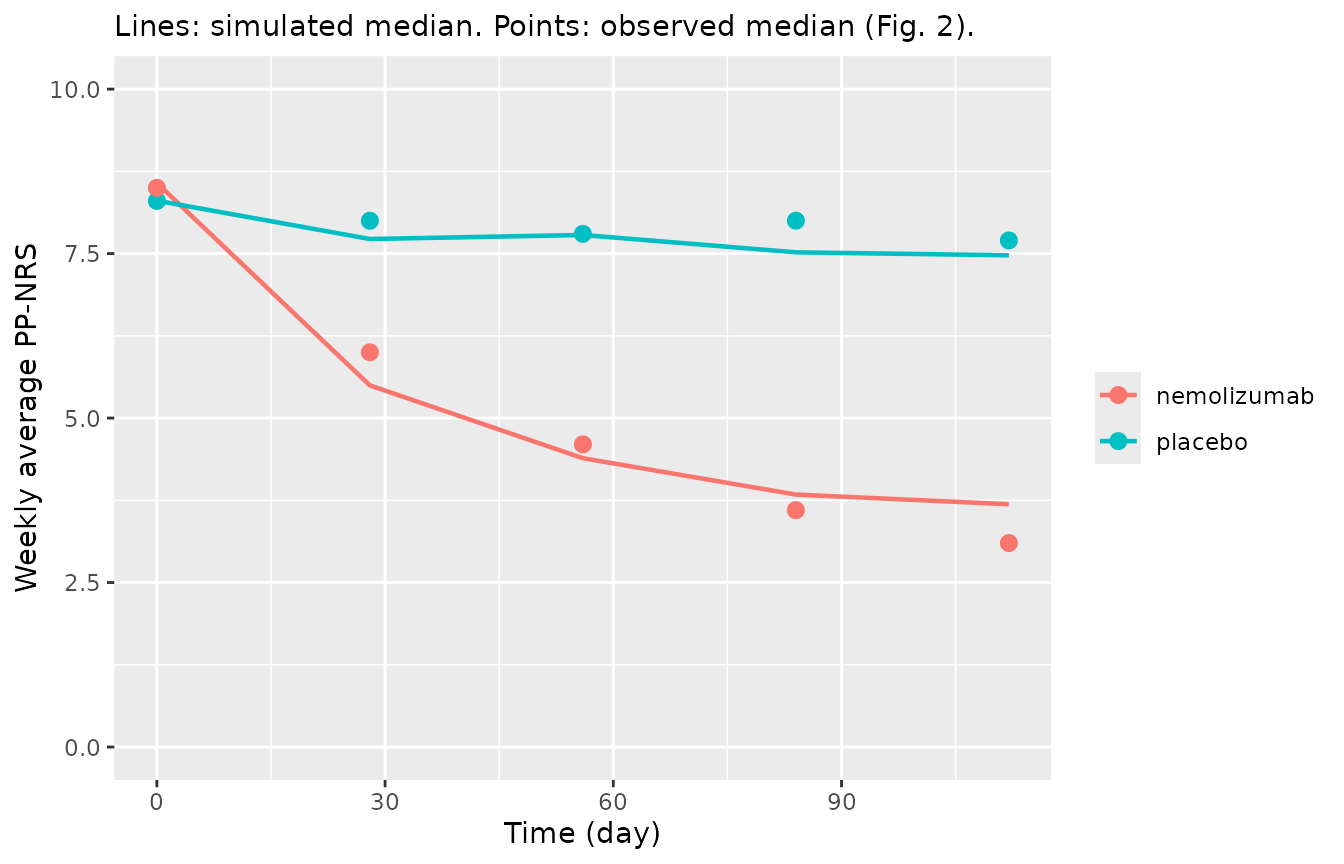
Simulated median PP-NRS (lines) against the observed medians read from Takechi 2025 Fig. 2 (points).
Onset rates
The paper’s rapid-onset claim is a statement about Kd
relative to Kp.
onset <- tibble::tibble(
  effect          = c("placebo", "nemolizumab"),
  `rate (1/day)`  = c(2.74e-3, 28.7e-3),
  `half-life (d)` = log(2) / c(2.74e-3, 28.7e-3),
  `% of maximum expressed by day 112` = 100 * (1 - exp(-c(2.74e-3, 28.7e-3) * 112))
)
knitr::kable(onset, digits = 1, caption = "Onset of the placebo and nemolizumab effects.")| effect | rate (1/day) | half-life (d) | % of maximum expressed by day 112 |
|---|---|---|---|
| placebo | 0 | 253.0 | 26.4 |
| nemolizumab | 0 | 24.2 | 96.0 |
stopifnot(
  abs(28.7e-3 / 2.74e-3 - 10.5) < 0.1,                       # deterministic
  onset$`% of maximum expressed by day 112`[2] > 95,
  onset$`% of maximum expressed by day 112`[1] < 30
)
Only about a quarter of the placebo maximum is expressed within the 112-day observation window, against essentially all of the nemolizumab maximum. That asymmetry – not the ratio of the maxima alone – is what produces the roughly eight-fold separation between the two arms in Fig. 2.
Part 3 – Model-based meta-analysis of IGA success rates
This model is a study-arm-level model. Its output is the proportion of an arm achieving at least a 2-point decrease in IGA, not an individual patient’s outcome, and its only random effect is between-study.
Reproducing Figure 4
Fig. 4B plots the typical (population-mean) time course of the IGA success rate for placebo, dupilumab and nemolizumab, and Fig. 4D gives simulated medians at weeks 4 and 16. With the between-study eta zeroed, the model is deterministic, so these are exact regression tests.
mbma0 <- rxode2::zeroRe(mbma)
#> Warning: No sigma parameters in the model

arms <- tibble::tribble(
  ~arm,          ~DOSE_NEMOLIZUMAB_MG, ~DOSE_DUPILUMAB_MG,
  "placebo",     0,                    0,
  "dupilumab",   0,                    300,
  "nemolizumab", 30,                   0
)
weeks <- c(4, 16, 24)

d_mbma <- arms |>
  dplyr::mutate(id = dplyr::row_number()) |>
  tidyr::crossing(time = weeks) |>
  dplyr::mutate(evid = 0L, amt = 0) |>
  dplyr::arrange(id, time)

sim_mbma <- as.data.frame(rxode2::rxSolve(mbma0, as.data.frame(d_mbma)))
#> ℹ omega/sigma items treated as zero: 'eta_study_eff'
#> Warning: multi-subject simulation without without 'omega'
sim_mbma$arm <- arms$arm[sim_mbma$id]

fig4 <- sim_mbma |>
  dplyr::transmute(Arm = arm, Week = time, `Model (%)` = 100 * pResp) |>
  dplyr::left_join(
    tibble::tribble(
      ~Arm,          ~Week, ~`Read from Fig. 4 (%)`,
      "placebo",     4,     2.5,
      "placebo",     16,    8.8,
      "placebo",     24,    11.0,
      "dupilumab",   4,     4.0,
      "dupilumab",   16,    26.5,
      "dupilumab",   24,    34.0,
      "nemolizumab", 4,     8.5,
      "nemolizumab", 16,    34.0,
      "nemolizumab", 24,    41.0
    ), by = c("Arm", "Week")
  ) |>
  dplyr::mutate(`Difference (points)` = `Model (%)` - `Read from Fig. 4 (%)`)
knitr::kable(fig4, digits = 1,
caption = "IGA success rate: model vs values read from Takechi 2025 Figs. 4B and 4D.")| Arm | Week | Model (%) | Read from Fig. 4 (%) | Difference (points) |
|---|---|---|---|---|
| placebo | 4 | 2.3 | 2.5 | -0.2 |
| placebo | 16 | 8.7 | 8.8 | -0.1 |
| placebo | 24 | 11.0 | 11.0 | 0.0 |
| dupilumab | 4 | 4.1 | 4.0 | 0.1 |
| dupilumab | 16 | 26.3 | 26.5 | -0.2 |
| dupilumab | 24 | 34.2 | 34.0 | 0.2 |
| nemolizumab | 4 | 8.5 | 8.5 | 0.0 |
| nemolizumab | 16 | 34.5 | 34.0 | 0.5 |
| nemolizumab | 24 | 40.7 | 41.0 | -0.3 |
# Deterministic (zeroRe), so the only error is figure read-off. A
# mis-transcribed theta moves these by many percentage points.
stopifnot(nrow(fig4) == 9L, max(abs(fig4$`Difference (points)`)) < 1.5)
Nine independent points across three arms and three time points are reproduced to within figure read-off precision, which validates the intercept, the placebo maximum and rate, and both drugs’ maxima and rates simultaneously.
d_curve <- arms |>
  dplyr::mutate(id = dplyr::row_number()) |>
  tidyr::crossing(time = seq(0, 24, by = 0.5)) |>
  dplyr::mutate(evid = 0L, amt = 0) |>
  dplyr::arrange(id, time)
curve <- as.data.frame(rxode2::rxSolve(mbma0, as.data.frame(d_curve)))
#> ℹ omega/sigma items treated as zero: 'eta_study_eff'
#> Warning: multi-subject simulation without without 'omega'
curve$arm <- arms$arm[curve$id]

ggplot(curve, aes(time, 100 * pResp, colour = arm)) +
  geom_line(linewidth = 0.8) +
  ylim(0, 80) +
  labs(x = "Time (week)", y = "IGA success rate (%)", colour = NULL)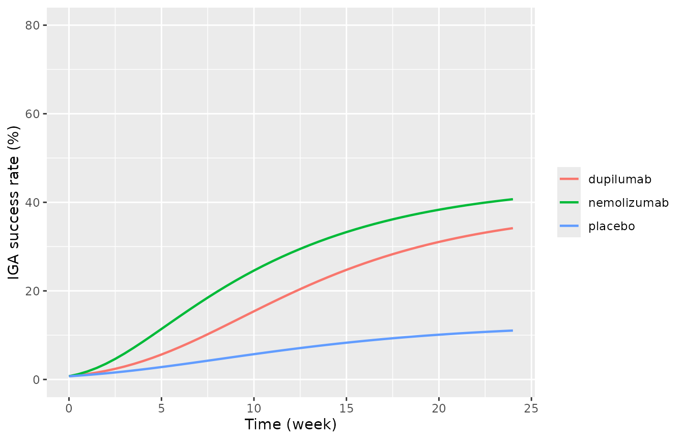
Typical IGA success-rate time courses. Replicates Figure 4B of Takechi 2025.
Nemolizumab is above dupilumab throughout, and the gap is widest early: at week 4 the model gives
early <- fig4 |> dplyr::filter(Week == 4) |> dplyr::select(Arm, `Model (%)`)
knitr::kable(early, digits = 1, caption = "Week-4 IGA success rate.")| Arm | Model (%) |
|---|---|
| placebo | 2.3 |
| dupilumab | 4.1 |
| nemolizumab | 8.5 |
nemo4 <- early$`Model (%)`[early$Arm == "nemolizumab"]
dupi4 <- early$`Model (%)`[early$Arm == "dupilumab"]
stopifnot(nemo4 > 2 * dupi4)   # deterministic
which is the quantitative content of the paper’s “particularly
notable rapid onset of effects during the early treatment phase”. It is
driven by the onset rate constants, not by the maxima: nemolizumab’s
Kd is 0.416/week against dupilumab’s 0.134/week, while its
maximum effect (1.71) is only slightly larger than dupilumab’s
(1.49).
Arm-size weighting of the residual
The paper’s residual is scaled by the binomial standard error of the
arm: success rate = Pr + eps * sqrt(Pr * (1 - Pr) / N). The
model encodes the prediction-dependent factor
sqrt(Pr * (1 - Pr)) exactly but ships the
N = 1 residual, because N is a property of the
arm being simulated rather than of the model – the same convention as
Boucher_2018_naproxen_mbma. Divide by
sqrt(N_arm) to reproduce a real arm.
set.seed(7)
n_rep  <- 400L
N_arm  <- 190L   # OLYMPIA 1 nemolizumab arm (Table 3)

d_rep <- data.frame(id = seq_len(n_rep), time = 24,
                    DOSE_NEMOLIZUMAB_MG = 30, DOSE_DUPILUMAB_MG = 0,
                    evid = 0L, amt = 0)
rep_sim <- as.data.frame(rxode2::rxSolve(mbma0, d_rep, nSub = n_rep))
#> ℹ omega/sigma items treated as zero: 'eta_study_eff'
#> Warning: multi-subject simulation without without 'omega'

sd_shipped  <- sd(rep_sim$sim)
sd_expected <- sqrt(0.619) * sqrt(mean(rep_sim$pResp) * (1 - mean(rep_sim$pResp)))
sd_for_arm  <- sd_shipped / sqrt(N_arm)

tibble::tibble(
  quantity = c("simulated residual SD (N = 1)",
               "expected addSd * sqrt(Pr(1-Pr))",
               paste0("rescaled for an arm of N = ", N_arm)),
  value    = c(sd_shipped, sd_expected, sd_for_arm)
) |>
knitr::kable(digits = 4, caption = "Residual SD of the shipped model and its per-arm rescaling.")| quantity | value |
|---|---|
| simulated residual SD (N = 1) | 0.3865 |
| expected addSd * sqrt(Pr(1-Pr)) | 0.3865 |
| rescaled for an arm of N = 190 | 0.0280 |
Part 4 – Model-based meta-analysis of PP-NRS success rates
The same six trials, the same logistic structure, the second endpoint: the proportion of an arm achieving at least a 4-point improvement in the weekly average PP-NRS. Two things differ from Part 3. The onset rate constants are far more separated (nemolizumab 1.93/week against dupilumab 0.119/week, a factor of sixteen, versus a factor of three for IGA), and this endpoint retains a covariate.
The covariate and its functional form
Table 4’s PP-NRS column carries a row absent from the IGA column:
PPM effect on Edrug,nemolizumab = -1.84, where
PPM is the paper’s abbreviation for the proportion of
patients classified as moderate by IGA in a study arm. It is
registered here as IGA_MOD_PCT, an arm-level percentage,
and is the complement of Table 3’s IGA4 at baseline (%)
column.
arm_ppm <- tibble::tibble(
  iga4_pct = c(46.1, 54.5, 52.6, 39.0, 53.0, 35.4, 43.7, 47.3, 41.0,
               29.3, 28.0, 39.5, 37.2)
) |>
  dplyr::mutate(IGA_MOD_PCT = 100 - iga4_pct)

ppm_median <- median(arm_ppm$IGA_MOD_PCT)
cat("13 arms; IGA_MOD_PCT range",
    sprintf("%.1f-%.1f%%", min(arm_ppm$IGA_MOD_PCT), max(arm_ppm$IGA_MOD_PCT)),
    "median", sprintf("%.1f%%", ppm_median), "\n")
#> 13 arms; IGA_MOD_PCT range 45.5-72.0% median 59.0%

# The centring constant hardcoded in model() must be the Table 3 median.
stopifnot(nrow(arm_ppm) == 13L, ppm_median == 59.0)
The paper never prints the covariate equation. Only the coefficient is given. The form encoded in the model file is a fractional deviation centred on that median arm,
and it was chosen because it is the only one of three candidate
readings that reproduces the paper’s own Fig. 4. Fig. 4’s caption states
the simulation used “the recommended dose of each drug in
Japan”, i.e. the Yokozeki 30 mg Q4W arm, whose
IGA_MOD_PCT is 100 - 54.5 = 45.5. That fixes
the covariate value and makes the three readings testable against three
plotted numbers.
# Closed-form logistic prediction, independent of the shipped model, so this
# genuinely discriminates between the candidate forms.
pr_ppnrs <- function(week, edrug_nemo) {
  f0 <- -4.38 + 2.64 * (1 - exp(-0.277 * week))
  100 * plogis(f0 + edrug_nemo * (1 - exp(-1.93 * week)))
}
ppm_ref  <- 0.455          # Yokozeki nemolizumab 30 mg Q4W arm
ppm_cent <- 0.590          # Table 3 median

candidates <- tibble::tibble(
  Form = c("fractional deviation (shipped)", "normalised power",
           "additive logit shift", "no covariate"),
  Edrug = c(1.63 * (1 - 1.84 * (ppm_ref - ppm_cent)),
            1.63 * (ppm_ref / ppm_cent)^(-1.84),
            1.63 - 1.84 * (ppm_ref - ppm_cent),
            1.63)
) |>
  dplyr::mutate(
    `Week 4 (%)`  = pr_ppnrs(4,  Edrug),
    `Week 16 (%)` = pr_ppnrs(16, Edrug),
    `Week 24 (%)` = pr_ppnrs(24, Edrug)
  )

knitr::kable(candidates, digits = 2,
             caption = paste("Candidate covariate forms for the nemolizumab arm of Fig. 4.",
                             "Fig. 4C reads ~36% at week 4 and ~56% at week 16;",
"the Fig. 4A plateau is ~57%."))| Form | Edrug | Week 4 (%) | Week 16 (%) | Week 24 (%) |
|---|---|---|---|---|
| fractional deviation (shipped) | 2.03 | 35.94 | 56.55 | 57.24 |
| normalised power | 2.63 | 50.40 | 70.22 | 70.80 |
| additive logit shift | 1.88 | 32.43 | 52.67 | 53.37 |
| no covariate | 1.63 | 27.24 | 46.47 | 47.17 |
shipped <- candidates[candidates$Form == "fractional deviation (shipped)", ]
# Deterministic arithmetic on transcribed thetas -- exact, not cohort-derived.
stopifnot(
  abs(shipped$`Week 4 (%)`  - 36) < 2,
  abs(shipped$`Week 16 (%)` - 56) < 2,
  abs(shipped$`Week 24 (%)` - 57) < 2
)
# ... and every alternative must MISS at week 24, or the test proves nothing.
others <- candidates[candidates$Form != "fractional deviation (shipped)", ]
stopifnot(all(abs(others$`Week 24 (%)` - 57) > 3))
The power function – the form the paper’s Methods states for the PopPD analysis – overshoots by 14 percentage points, the additive shift undershoots by 4, and dropping the covariate undershoots by 10. Only the fractional deviation lands. This is a reconstruction, and it is recorded as one in the model file and in the Assumptions below.
Reproducing Figure 4A and 4C
With the covariate form settled, the placebo and dupilumab arms are an independent check: neither carries the covariate, so if the rest of the column were mis-transcribed they would miss too.
mbma_p0 <- rxode2::zeroRe(mbma_ppnrs)
#> Warning: No sigma parameters in the model

arms_p <- tibble::tribble(
  ~arm,          ~DOSE_NEMOLIZUMAB_MG, ~DOSE_DUPILUMAB_MG, ~IGA_MOD_PCT,
  "placebo",     0,                    0,                  45.5,
  "dupilumab",   0,                    300,                45.5,
  "nemolizumab", 30,                   0,                  45.5
)

d_p <- arms_p |>
  dplyr::mutate(id = dplyr::row_number()) |>
  tidyr::crossing(time = c(4, 16, 24)) |>
  dplyr::mutate(evid = 0L, amt = 0) |>
  dplyr::arrange(id, time)

sim_p <- as.data.frame(rxode2::rxSolve(mbma_p0, as.data.frame(d_p)))
#> ℹ omega/sigma items treated as zero: 'eta_study_eff'
#> Warning: multi-subject simulation without without 'omega'
sim_p$arm <- arms_p$arm[sim_p$id]

fig4a <- sim_p |>
  dplyr::transmute(Arm = arm, Week = time, `Model (%)` = 100 * pResp) |>
  dplyr::left_join(
    tibble::tribble(
      ~Arm,          ~Week, ~`Read from Fig. 4 (%)`,
      "placebo",     4,     7,
      "placebo",     16,    14,
      "placebo",     24,    15,
      "dupilumab",   4,     13,
      "dupilumab",   16,    46,
      "dupilumab",   24,    52,
      "nemolizumab", 4,     36,
      "nemolizumab", 16,    56,
      "nemolizumab", 24,    57
    ), by = c("Arm", "Week")
  ) |>
  dplyr::mutate(`Difference (points)` = `Model (%)` - `Read from Fig. 4 (%)`)

knitr::kable(fig4a, digits = 1,
caption = "PP-NRS success rate: model vs values read from Takechi 2025 Figs. 4A and 4C.")| Arm | Week | Model (%) | Read from Fig. 4 (%) | Difference (points) |
|---|---|---|---|---|
| placebo | 4 | 6.8 | 7 | -0.2 |
| placebo | 16 | 14.5 | 14 | 0.5 |
| placebo | 24 | 14.9 | 15 | -0.1 |
| dupilumab | 4 | 13.2 | 13 | 0.2 |
| dupilumab | 16 | 46.8 | 46 | 0.8 |
| dupilumab | 24 | 51.9 | 52 | -0.1 |
| nemolizumab | 4 | 35.9 | 36 | -0.1 |
| nemolizumab | 16 | 56.5 | 56 | 0.5 |
| nemolizumab | 24 | 57.2 | 57 | 0.2 |
# Deterministic (zeroRe), so the only error is figure read-off. The week-4 and
# week-16 targets are the open and closed circles of the Fig. 4C forest plot;
# the week-24 targets are the right-hand end of the Fig. 4A curves. These were
# read off a 150 dpi render of the publisher's page and are good to roughly a
# point, so the gate is set at 2 -- still far tighter than the many-point shift
# a mis-transcribed theta produces.
stopifnot(nrow(fig4a) == 9L, max(abs(fig4a$`Difference (points)`)) < 2)
d_pc <- arms_p |>
  dplyr::mutate(id = dplyr::row_number()) |>
  tidyr::crossing(time = seq(0, 24, by = 0.5)) |>
  dplyr::mutate(evid = 0L, amt = 0) |>
  dplyr::arrange(id, time)
curve_p <- as.data.frame(rxode2::rxSolve(mbma_p0, as.data.frame(d_pc)))
#> ℹ omega/sigma items treated as zero: 'eta_study_eff'
#> Warning: multi-subject simulation without without 'omega'
curve_p$arm <- arms_p$arm[curve_p$id]

ggplot(curve_p, aes(time, 100 * pResp, colour = arm)) +
  geom_line(linewidth = 0.8) +
  ylim(0, 80) +
  labs(x = "Time (week)", y = "PP-NRS success rate (%)", colour = NULL)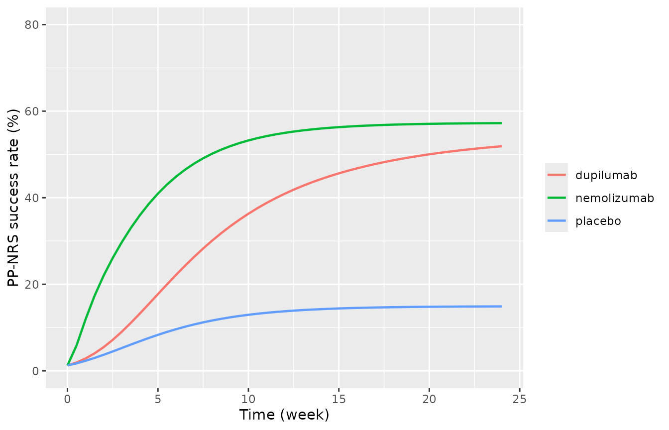
Typical PP-NRS success-rate time courses for the Yokozeki 30 mg Q4W arm severity. Replicates Figure 4A of Takechi 2025.
The nemolizumab curve is essentially at its plateau by week 4 while dupilumab is still climbing at week 24 – the clearest quantitative statement in the paper of the rapid-itch-relief claim, and a much starker separation than the IGA endpoint of Part 3 shows.
Covariate direction across the observed arm range
A lower IGA_MOD_PCT means a more severe arm, and the
negative coefficient makes such an arm respond more. The effect is not
small over the range the meta-analysis actually spans.
d_cov <- tibble::tibble(IGA_MOD_PCT = sort(arm_ppm$IGA_MOD_PCT)) |>
  dplyr::mutate(id = dplyr::row_number(),
                DOSE_NEMOLIZUMAB_MG = 30, DOSE_DUPILUMAB_MG = 0,
                time = 24, evid = 0L, amt = 0)

cov_sim <- as.data.frame(rxode2::rxSolve(mbma_p0, as.data.frame(d_cov)))
#> ℹ omega/sigma items treated as zero: 'eta_study_eff'
#> Warning: multi-subject simulation without without 'omega'
cov_sim$IGA_MOD_PCT <- d_cov$IGA_MOD_PCT[cov_sim$id]

cov_tab <- cov_sim |>
  dplyr::transmute(`Arm moderate-IGA (%)` = IGA_MOD_PCT,
                   `Week-24 success (%)`  = 100 * pResp)
knitr::kable(cov_tab, digits = 1,
caption = "Week-24 nemolizumab PP-NRS success rate across the 13 arms' observed severity range.")| Arm moderate-IGA (%) | Week-24 success (%) |
|---|---|
| 45.5 | 57.2 |
| 47.0 | 56.1 |
| 47.4 | 55.8 |
| 52.7 | 51.9 |
| 53.9 | 51.0 |
| 56.3 | 49.2 |
| 59.0 | 47.2 |
| 60.5 | 46.0 |
| 61.0 | 45.7 |
| 62.8 | 44.3 |
| 64.6 | 43.0 |
| 70.7 | 38.6 |
| 72.0 | 37.7 |
Arm-size weighting of the residual
Identical convention to Part 3: the model ships the
N = 1 residual and the 1 / sqrt(N_arm) factor
is applied downstream.
set.seed(11)
n_rep_p <- 400L
N_arm_p <- 77L   # Yokozeki nemolizumab 30 mg Q4W arm (Table 3)

d_rep_p <- data.frame(id = seq_len(n_rep_p), time = 24,
                      DOSE_NEMOLIZUMAB_MG = 30, DOSE_DUPILUMAB_MG = 0,
                      IGA_MOD_PCT = 45.5, evid = 0L, amt = 0)
rep_p <- as.data.frame(rxode2::rxSolve(mbma_p0, d_rep_p, nSub = n_rep_p))
#> ℹ omega/sigma items treated as zero: 'eta_study_eff'
#> Warning: multi-subject simulation without without 'omega'

sd_shipped_p  <- sd(rep_p$sim)
sd_expected_p <- sqrt(0.738) * sqrt(mean(rep_p$pResp) * (1 - mean(rep_p$pResp)))
sd_for_arm_p  <- sd_shipped_p / sqrt(N_arm_p)

tibble::tibble(
  quantity = c("simulated residual SD (N = 1)",
               "expected addSd * sqrt(Pr(1-Pr))",
               paste0("rescaled for an arm of N = ", N_arm_p)),
  value    = c(sd_shipped_p, sd_expected_p, sd_for_arm_p)
) |>
knitr::kable(digits = 4, caption = "Residual SD of the shipped PP-NRS model and its per-arm rescaling.")| quantity | value |
|---|---|
| simulated residual SD (N = 1) | 0.4045 |
| expected addSd * sqrt(Pr(1-Pr)) | 0.4250 |
| rescaled for an arm of N = 77 | 0.0461 |
Assumptions and deviations
1. Pmax and Edrug of the PopPD
model are read as log-scale thetas. Table 2 prints them without
units while labelling Kp and Kd
(x 10^-3/day). The evidence is set out in full in the
“Reading Pmax and Edrug” section above and in the model file: a unitless
column, an unrescuable 3.7-point miss of the Fig. 2 active-arm median
under the linear reading, a matching 50th and 95th percentile under the
log-scale reading, and the paper’s own statement that its simulated 5th
percentile ran too low. The paper never states the scale explicitly, so
this is an inference, but it is a figure-falsified one rather than a
preference.
2. The PopPD equation that combines the two response
components with the baseline is not printed in the paper.
Methods “Pharmacodynamic Model” gives Placebo response(t)
and Drug response(t) but no line assembling them into a
PP-NRS prediction. The additive assembly used here –
PP-NRS = baseline - placebo response - drug response –
follows from the paper’s own definition of Pmax and
Edrug as “the maximum effects, defined as the reduction
in PP-NRS scores” and is what reproduces Fig. 2. This is a genuine
reporting gap in the source, not a text-extraction loss: the PDF, the
PMC full-text XML and the supplement all contain only the two component
equations.
3. Variance-vs-SD reading of the variability rows.
Table 2’s IIV rows are variances, proved above from the CL/F-V/F
covariance row. The same convention is applied to Table 2’s
Additive error (0.582 -> SD 0.763) and Table 4’s
ISV on EFF and Additive error, on the grounds
that every row in those tables is on the raw NONMEM scale except the one
the authors explicitly relabelled log normal error (CV%).
Reading Table 2’s additive error instead as an SD of 0.582 changes the
residual by 24% and no structural conclusion; a user who prefers that
reading can set addSd = 0.582.
4. Serum albumin units. Table 1 heads the albumin
row “Serum albumin (g/L)” but tabulates 4.3-4.5 with a range of 2.0-5.2.
Those are g/dL: 45 g/L is a normal serum albumin and
4.5 g/L is not survivable, and the model equation’s own reference of 4.5
confirms it. The Table 1 header is a publication unit-label error. The
covariate register stores ALB in SI g/L, so the model
applies the register’s documented inline conversion
alb_gdL <- ALB * 0.1 before the power term.
5. Allometric exponents are fixed().
Neither 0.75 nor the implicit 1 on V/F appears as an estimated row in
Table 2 with an %RSE or a bootstrap CI; both are printed only inside the
displayed equations, so both are encoded as structural assumptions.
6. Observed percentiles in Part 2 and the Fig. 4 values in
Part 3 are read from figures. The paper tabulates neither, so
the comparison targets were read off Fig. 2 and Figs. 4B/4D at the
resolution of the publisher’s figure files. The gates are set to
tolerate read-off error (1.5 points / 1.5 percentage points) while still
failing on a mis-transcribed parameter, which moves these quantities by
many points. No parameter value in any model file is figure-derived –
every ini() entry comes from Table 2 or Table 4.
7. The MBMA residual ships at N = 1.
See “Arm-size weighting” above.
8. No PK-PD link. The PopPD and MBMA models take no concentration input. This is the authors’ structure, not a simplification: no exposure-response relationship was identifiable, so the drug effects are constants selected by a dose column used only as an on/off switch.
9. No 0-10 floor on the PP-NRS prediction. The source describes no clamping, and clamping would change the residual distribution near zero. Simulated values below 0 occur for strong responders and are visible in the paper’s own Fig. 2, whose lower prediction band sits against the axis.
10. Simulation scope. Both
Takechi_2025_nemolizumab_mbma_iga and
Takechi_2025_nemolizumab_mbma_ppnrs predict study-arm
success rates and must not be used to simulate individual patients;
their only random effect is between-study.
Takechi_2025_nemolizumab_ppnrs does describe individual
subjects.
11. The PP-NRS covariate’s functional form is reconstructed,
not quoted. Table 4 prints the coefficient -1.84
but the paper contains no equation attaching PPM to
Edrug,nemolizumab anywhere – not in Methods, not in the
supplement, and no NONMEM control stream was available. The fractional
deviation 1.63 * (1 + (-1.84) * (IGA_MOD_PCT/100 - 0.590))
used here is the reading that reproduces three independent plotted
values of Fig. 4, where the two obvious alternatives miss by 14 and 4
percentage points respectively; Part 4 runs that discrimination as a
test. The centring constant 0.590 is likewise not printed –
it is the median of Table 3’s 13 arms, which the vignette recomputes and
asserts. A reader who has access to the authors’ control stream should
check this term before relying on the model outside the 45.5-72.0%
severity range the meta-analysis spans.
12. IGA_MOD_PCT scale. The covariate
register stores this column as a percent (0-100),
matching its arm-level siblings TUMTP_SQUAM_PCT,
PS_ECOG_0_PCT and RACE_ASIAN_PCT; the model
converts to a fraction inline. The paper’s PPM is a
fraction, so a user transcribing directly from Table 4’s notation must
multiply by 100 before supplying the column.
Session info
sessionInfo()
#> R version 4.6.1 (2026-06-24)
#> Platform: x86_64-pc-linux-gnu
#> Running under: Ubuntu 24.04.5 LTS
#>
#> Matrix products: default
#> BLAS:   /usr/lib/x86_64-linux-gnu/openblas-pthread/libblas.so.3
#> LAPACK: /usr/lib/x86_64-linux-gnu/openblas-pthread/libopenblasp-r0.3.26.so;  LAPACK version 3.12.0
#>
#> locale:
#>  [1] LC_CTYPE=C.UTF-8       LC_NUMERIC=C           LC_TIME=C.UTF-8
#>  [4] LC_COLLATE=C.UTF-8     LC_MONETARY=C.UTF-8    LC_MESSAGES=C.UTF-8
#>  [7] LC_PAPER=C.UTF-8       LC_NAME=C              LC_ADDRESS=C
#> [10] LC_TELEPHONE=C         LC_MEASUREMENT=C.UTF-8 LC_IDENTIFICATION=C
#>
#> time zone: UTC
#> tzcode source: system (glibc)
#>
#> attached base packages:
#> [1] stats     graphics  grDevices utils     datasets  methods   base
#>
#> other attached packages:
#> [1] ggplot2_4.0.3         tidyr_1.3.2           dplyr_1.2.1
#> [4] PKNCA_0.12.1          rxode2_5.1.8          nlmixr2lib_0.3.2.9000
#>
#> loaded via a namespace (and not attached):
#>  [1] gtable_0.3.6        xfun_0.61           bslib_0.12.0
#>  [4] rxode2lincmt_0.1.0  lattice_0.22-9      vctrs_0.7.3
#>  [7] tools_4.6.1         generics_0.1.4      parallel_4.6.1
#> [10] tibble_3.3.1        symengine_0.2.13    pkgconfig_2.0.3
#> [13] data.table_1.18.6.1 checkmate_2.3.4     RColorBrewer_1.1-3
#> [16] S7_0.2.2            desc_1.4.3          lifecycle_1.0.5
#> [19] compiler_4.6.1      farver_2.1.2        textshaping_1.0.5
#> [22] fontawesome_0.5.3   htmltools_0.5.9     sys_3.4.3
#> [25] sass_0.4.10         yaml_2.3.12         pillar_1.11.1
#> [28] pkgdown_2.2.1       crayon_1.5.3        jquerylib_0.1.4
#> [31] whisker_0.4.1       openssl_2.4.2       cachem_1.1.0
#> [34] nlme_3.1-169        tidyselect_1.2.1    digest_0.6.39
#> [37] lotri_1.0.5         purrr_1.2.2         labeling_0.4.3
#> [40] rxode2ll_2.0.18     fastmap_1.2.0       grid_4.6.1
#> [43] cli_3.6.6           dparser_1.3.1-13    magrittr_2.0.5
#> [46] withr_3.0.3         scales_1.4.0        backports_1.5.1
#> [49] rmarkdown_2.32      otel_0.2.0          askpass_1.2.1
#> [52] ragg_1.5.2          memoise_2.0.1       evaluate_1.0.5
#> [55] knitr_1.52          rex_1.2.2           PreciseSums_0.7
#> [58] rlang_1.3.0         downlit_0.4.5       Rcpp_1.1.2
#> [61] glue_1.8.1          xml2_1.6.0          jsonlite_2.0.0
#> [64] R6_2.6.1            systemfonts_1.3.2   fs_2.1.0