Selpercatinib (Liu 2025)
Source:vignettes/articles/Liu_2025_selpercatinib.Rmd
Liu_2025_selpercatinib.RmdModel and source
- Citation: Liu D, van der Walt JS. (2025). Population pharmacokinetics modeling of selpercatinib to support posology in pediatric patients with RET-altered metastatic thyroid cancer or solid tumors. CPT Pharmacometrics Syst Pharmacol 14(11):1848-1857. doi:10.1002/psp4.70042
- Description: Two-compartment population PK model for selpercatinib (RETEVMO, a first-in-class highly selective RET kinase inhibitor approved for RET-altered lung, thyroid and other solid tumors) in adult, adolescent and pediatric patients (Liu 2025; N = 830 patients, 8024 plasma concentrations pooled from the phase 1/2 studies LIBRETTO-001 in patients aged 12 years and older and LIBRETTO-121 in patients aged 6 months to 21 years). Absorption is sequential zero-order then first-order: the oral dose enters the gut depot over a zero-order window Dur = 1.09 h and the depot then drains first-order at ka = 1.47 1/h. Disposition is two-compartment with first-order elimination; typical apparent values for a 70 kg patient at the 160 mg reference dose are CL/F = 6.04 L/h, Vc/F = 99.6 L, Q/F = 29.6 L/h and Vp/F = 91.3 L. Relative bioavailability F1 is fixed to 1 and carries the only non-weight covariate on absorption: Asian race raises F1 by 18.3%. Body weight enters allometrically with the standard fixed exponents referenced to 70 kg (0.75 on CL/F and Q/F, 1 on Vc/F and Vp/F). The administered dose acts on CL/F as a time-varying linear covariate centered on 160 mg, -0.321% per mg, so apparent clearance falls as the dose rises and exposure is more than dose proportional over the 20-240 mg range studied. Baseline age, sex, creatinine clearance, liver function tests and concomitant medication were screened and not retained; an age effect on CL/F was statistically significant but was removed during model refinement because it biased predictions in children. Inter-individual variability is estimated on CL/F (48.8%), Vc/F (66.1%), ka (63.6%) and Dur (56.2%); residual error is proportional (25.3%) plus additive (61.5 ng/mL).
- Article: https://doi.org/10.1002/psp4.70042
- Supplement (Tables S1-S3, Figures S1-S7): https://doi.org/10.1002/psp4.70042 (Supporting
Information,
PSP4-14-1848-s001.docx)
Selpercatinib is a highly selective RET kinase inhibitor. Liu 2025 updated a previously developed adult population PK model with pediatric data in order to choose a pediatric dose regimen by matching exposure to that of adults treated at the approved 160 mg twice-daily dose. The resulting regimen (Table 3 of the paper) was granted FDA accelerated approval for patients 2 years and older on 29 May 2024.
Population
The analysis pooled two ongoing open-label phase 1/2 studies with a data cut-off of 13 January 2023 (Liu 2025 Methods “Study Design”, Table 1):
- LIBRETTO-001 (NCT03157128), patients aged 12 years and older with advanced or metastatic solid tumors: 803 patients contributing 7723 concentrations. Doses ranged from 20 mg once daily to 240 mg twice daily during phase 1 dose escalation; phase 2 used 160 mg twice daily.
- LIBRETTO-121 (NCT03899792), patients enrolled from 6 months to 21 years of age with an activating RET alteration and an advanced solid or primary CNS tumor: 27 patients contributing 301 concentrations, dosed on body surface area (92 mg/m^2 twice daily, capped at 160 mg twice daily).
Overall 830 patients contributed 8024 concentrations. Median age was 58.0 years (range 2.0-92.0), median weight 67.0 kg (range 9.6-179) and median BSA 1.76 m^2 (range 0.446-2.79); 403/830 (48.6%) were female. Only 6 patients (0.7%) were under 12 years of age and they contributed just 59 concentrations, which the Discussion identifies as the analysis’s principal limitation. A further 133 concentrations were below the 1 ng/mL assay limit of quantification and were excluded.
Liu 2025 Table 1 does not report the race distribution, even though Asian race is a covariate in the final model; see Assumptions below.
The same information is available programmatically via the model’s
population metadata
(readModelDb("Liu_2025_selpercatinib")()$population).
Source trace
Every ini() entry carries an in-file comment naming its
origin in
inst/modeldb/specificDrugs/Liu_2025_selpercatinib.R. They
are collected here for review. All final estimates come from Liu 2025
Table 2, “NONMEM parameter estimates for the final model”; the covariate
functions are printed in the “Functions and Parameters Used to Test
Covariates” block of that same table.
| Equation / parameter | Value | Source location |
|---|---|---|
lcl = log CL/F |
log(6.04) L/h | Table 2 CL (L/h) = 6.04 (95% CI 5.79/6.29) |
lvc = log Vc/F |
log(99.6) L | Table 2 Vc (L) = 99.6 (86.3/113) |
lvp = log Vp/F |
log(91.3) L | Table 2 Vp (L) = 91.3 (82.9/99.7) |
lq = log Q/F |
log(29.6) L/h | Table 2 Q (L/h) = 29.6 (24.2/35.0) |
lka |
log(1.47) 1/h | Table 2 ka (1/h) = 1.47 (1.25/1.69) |
ld1 = log zero-order duration |
log(1.09) h | Table 2 Dur (h) = 1.09 (1.05/1.13) |
lfdepot = log F1 |
fixed(log(1)) |
Table 2 F1 (fraction) 1.00 Fixed; Figure 1 caption “F,
bioavailability (fixed to 100%)” |
e_wt_cl |
fixed(0.75) |
Methods “Population PK Analysis”; Table 2 covariate functions for CL and Q |
e_wt_vc |
fixed(1) |
Methods “Population PK Analysis”; Table 2 covariate functions for Vc and Vp |
e_dose_cl |
-0.00321 /mg | Table 2 Dose effect on CL (%/mg) = -0.321
(-0.439/-0.203), divided by 100 |
e_race_asian_fdepot |
0.183 | Table 2 Asian race effect on F1 (%) = 18.3 (10.9/25.8),
divided by 100 |
etalcl |
0.2136135 | Table 2 IIV on CL = 48.8%, as log(CV^2 + 1)
|
etalvc |
0.3625026 | Table 2 IIV on Vc = 66.1%, as log(CV^2 + 1)
|
etalka |
0.3396785 | Table 2 IIV on ka = 63.6%, as log(CV^2 + 1)
|
etald1 |
0.2744783 | Table 2 IIV on Dur = 56.2%, as log(CV^2 + 1)
|
addSd |
61.5 ng/mL | Table 2 Additive RUV (mg/L) = 61.5 (37.4/85.6); unit
tag read as ng/mL, see Errata |
propSd |
0.253 | Table 2 Proportional RUV (fraction) = 0.253
(0.231/0.275) |
Sequential zero- then first-order absorption;
dur(depot), then ka into
central
|
n/a | Figure 1 schematic; Abstract; Results “PK Analyses” |
| Two-compartment disposition, first-order elimination | n/a | Figure 1 schematic; Methods “Population PK Analysis” |
CL = theta_CL * (1 + theta_dose * (Dose - 160 mg)) * (WT/70)^0.75 |
n/a | Table 2 covariate-function block; Table S2 footnote (b) fixes the 160 mg centring |
F1 = theta_F1 * (1 + theta_Asian) |
n/a | Table 2 covariate-function block; Table S2 footnote (a) defines Asian vs non-Asian |
Vc = theta_Vc * (WT/70)^1.0,
Vp = theta_Vp * (WT/70)^1.0,
Q = theta_Q * (WT/70)^0.75
|
n/a | Table 2 covariate-function block |
| Recommended pediatric regimen simulated below | n/a | Table 3 “Recommended selpercatinib doses for patients aged 2-17 years” |
| Adult reference exposure targets | Cmax ~3 mg/L, AUC0-24 ~53 mg*h/L | Figures 3 and 4, orange dashed “Adult reference level” line (read off the figure) |
Closed-form gate on the typical-value model
Before any cohort is simulated, the structural model is checked
against the identity it must satisfy exactly. At steady state on a
regimen of dose D every tau hours, the area
under the curve over one dosing interval is F * D / CL,
independent of absorption, distribution and the number of compartments.
This is a pure numerical check on the solved ODEs – both sides use the
same parameters, so a tight bound is the right assertion here (unlike
the cohort assertions further down, which must be robust to which
subjects are drawn).
mod <- readModelDb("Liu_2025_selpercatinib")

# Typical 70 kg non-Asian adult on the approved 160 mg BID regimen, run out to
# 30 days so that the ~23 h terminal half-life is fully accumulated.
ev_typ <- rxode2::et(amt = 160, ii = 12, until = 24 * 30, rate = -2, cmt = "depot") |>
  rxode2::et(seq(24 * 29, 24 * 30, by = 0.02), cmt = "central") |>
  as.data.frame()
ev_typ$WT <- 70
ev_typ$DOSE <- 160
ev_typ$RACE_ASIAN <- 0

sim_typ <- rxode2::rxSolve(rxode2::zeroRe(mod), ev_typ, returnType = "data.frame")
#> ℹ parameter labels from comments will be replaced by 'label()'
#> ℹ omega/sigma items treated as zero: 'etalcl', 'etalvc', 'etalka', 'etald1'

# One dosing interval at the end of the run.
tau_win <- subset(sim_typ, time >= 24 * 29 + 12 & time <= 24 * 29 + 24)
auc_tau <- sum(diff(tau_win$time) *
                 (head(tau_win$Cc, -1) + tail(tau_win$Cc, -1)) / 2)
auc_closed <- 1 * 160 / 6.04 * 1000  # F * D / CL, in ng*h/mL

c(auc_solved = auc_tau, auc_closed_form = auc_closed,
  ratio = auc_tau / auc_closed)
#>      auc_solved auc_closed_form           ratio
#>        26490.07        26490.07            1.00
# The two sides share the drawn parameters, so the only difference is
# trapezoidal and accumulation error -- a tight bound is correct here.
stopifnot(abs(auc_tau / auc_closed - 1) < 0.005)
The covariate functions are likewise checked as exact algebra rather than eyeballed, using the per-subject parameters rxode2 returns alongside the concentrations.
grid <- expand.grid(WT = c(10, 30, 70, 120), DOSE = c(40, 120, 160, 240),
                    RACE_ASIAN = c(0, 1))
grid$id <- seq_len(nrow(grid))

ev_grid <- lapply(seq_len(nrow(grid)), function(i) {
  d <- rxode2::et(amt = grid$DOSE[i], ii = 12, until = 24, rate = -2, cmt = "depot") |>
    rxode2::et(c(0, 6, 12), cmt = "central") |>
    as.data.frame()
  d$id <- grid$id[i]
  d$WT <- grid$WT[i]
  d$DOSE <- grid$DOSE[i]
  d$RACE_ASIAN <- grid$RACE_ASIAN[i]
  d
}) |>
  dplyr::bind_rows()

sim_grid <- rxode2::rxSolve(rxode2::zeroRe(mod), ev_grid,
                            returnType = "data.frame") |>
  dplyr::distinct(id, .keep_all = TRUE) |>
  dplyr::left_join(grid, by = c("id", "WT", "DOSE", "RACE_ASIAN"))
#> ℹ parameter labels from comments will be replaced by 'label()'
#> ℹ omega/sigma items treated as zero: 'etalcl', 'etalvc', 'etalka', 'etald1'
#> Warning: multi-subject simulation without without 'omega'

chk <- sim_grid |>
  dplyr::mutate(
    cl_expected = 6.04 * (1 - 0.00321 * (DOSE - 160)) * (WT / 70)^0.75,
    vc_expected = 99.6 * (WT / 70),
    vp_expected = 91.3 * (WT / 70),
    q_expected  = 29.6 * (WT / 70)^0.75,
    f_expected  = 1 + 0.183 * RACE_ASIAN
  )

# Every covariate function must reproduce to machine precision.
stopifnot(
  max(abs(chk$cl / chk$cl_expected - 1)) < 1e-8,
  max(abs(chk$vc / chk$vc_expected - 1)) < 1e-8,
  max(abs(chk$vp / chk$vp_expected - 1)) < 1e-8,
  max(abs(chk$q  / chk$q_expected  - 1)) < 1e-8,
  max(abs(chk$fdepot / chk$f_expected - 1)) < 1e-8
)

# The dose effect reproduces the paper's direction and magnitude: apparent
# clearance falls as the dose rises, so exposure is more than dose
# proportional over the 20-240 mg range studied.
chk |>
  dplyr::filter(WT == 70, RACE_ASIAN == 0) |>
  dplyr::transmute(
    "Dose (mg)"          = DOSE,
    "CL/F (L/h)"         = round(cl, 3),
    "Multiplier vs 160 mg" = round(cl / 6.04, 4)
  ) |>
knitr::kable(caption = "Table 2 dose effect on CL/F, -0.321% per mg, centred on 160 mg.")| Dose (mg) | CL/F (L/h) | Multiplier vs 160 mg |
|---|---|---|
| 40 | 8.367 | 1.3852 |
| 120 | 6.816 | 1.1284 |
| 160 | 6.040 | 1.0000 |
| 240 | 4.489 | 0.7432 |
Virtual cohort
Original observed data are not publicly available. Liu 2025 drew its simulation covariates from the NHANES DXA database, which is not reproduced here; instead three arms are built whose covariate distributions match the published trial demographics and whose dose assignment follows the paper’s own rules.
# `set.seed()` seeds R's RNG, not rxode2's simulation streams (which are
# partitioned per solver thread), so this cohort is reproducible on one machine
# and different on a machine with a different thread count. Every assertion
# below is therefore written on medians and robust quantiles, never on the
# extremes of the drawn cohort.
set.seed(20250425)

N_PER_ARM <- 200L

# Growth reference used to turn an age into a weight and a height so that
# Mosteller BSA (and hence the Table 3 dose band) can be assigned. The weight
# curve is rescaled so that it passes through the LIBRETTO-121 median pair
# (14.0 years, 48.5 kg) from Liu 2025 Table 1; the height curve is a paediatric
# 50th-percentile reference. See Assumptions.
ref_age <- c(2, 3, 4, 5, 6, 8, 10, 12, 14, 16, 17)
ref_wt  <- c(12.5, 14.3, 16.3, 18.5, 20.8, 26.0, 32.5, 40.5, 50.0, 58.0, 61.0)
ref_ht  <- c(87, 96, 103, 110, 116, 128, 139, 150, 162, 170, 172)

wt_for_age <- function(age) exp(approx(log(ref_age), log(ref_wt), log(age), rule = 2)$y)
ht_for_age <- function(age) exp(approx(log(ref_age), log(ref_ht), log(age), rule = 2)$y)
wt_scale <- 48.5 / wt_for_age(14)

mosteller <- function(wt, ht) sqrt(wt * ht / 3600)

# Table 3 of Liu 2025: the recommended regimen for patients aged 2-17 years.
# 12 years and older is dosed on weight; 2 to under 12 years on BSA, with the
# 92 mg/m^2 target rounded to the available 40 and 80 mg capsules.
recommended_dose <- function(age, wt, bsa) {
  dplyr::case_when(
    age >= 12 & wt <  50 ~ 120,
    age >= 12 & wt >= 50 ~ 160,
    bsa >= 1.53          ~ 160,
    bsa >= 1.09          ~ 120,
    bsa >= 0.66          ~  80,
    TRUE                 ~  40   # BSA 0.33-0.65 m^2, given three times a day
  )
}
recommended_ii <- function(dose_mg) ifelse(dose_mg == 40, 8, 12)

# The comparator the paper rejected: adapted flat (adult weight-based) dosing
# applied to children as well.
flat_dose <- function(wt) ifelse(wt < 50, 120, 160)

make_peds <- function(n, regimen, id_offset = 0L) {
  age <- runif(n, 2, 17.99)
  wt  <- wt_for_age(age) * wt_scale * rlnorm(n, 0, 0.15)
  ht  <- ht_for_age(age) * rlnorm(n, 0, 0.04)
  bsa <- mosteller(wt, ht)
  amt <- if (regimen == "Recommended (Table 3)") {
    recommended_dose(age, wt, bsa)
  } else {
    flat_dose(wt)
  }
  tibble::tibble(
    id = id_offset + seq_len(n), AGE = age, WT = wt, BSA = bsa,
    DOSE = amt, ii = recommended_ii(amt), regimen = regimen,
    RACE_ASIAN = 0L
  )
}

# Adult reference arm: LIBRETTO-001 weight marginal (median 67.3 kg, SD 19.6,
# Liu 2025 Table 1) on the approved adult 160 mg BID regimen. Adults enter here
# only as the exposure target the pediatric regimen is matched to.
make_adults <- function(n, id_offset = 0L) {
  wt <- pmin(pmax(rlnorm(n, log(67.3), 0.27), 26.8), 179)
  tibble::tibble(
    id = id_offset + seq_len(n), AGE = NA_real_, WT = wt, BSA = NA_real_,
    DOSE = 160, ii = 12, regimen = "Adults 160 mg BID", RACE_ASIAN = 0L
  )
}

subjects <- dplyr::bind_rows(
  make_adults(N_PER_ARM, id_offset = 0L),
  make_peds(N_PER_ARM, "Recommended (Table 3)", id_offset = 1000L),
  make_peds(N_PER_ARM, "Adapted flat dosing",   id_offset = 2000L)
)

# Dose through the end of Cycle 1 Day 8 (day 1 spans 0-24 h, so day 8 spans
# 168-192 h), with a coarse grid through the accumulation phase and a fine grid
# across the C1D8 window that Figures 3 and 4 report.
build_records <- function(s) {
  dose_times <- seq(0, 192 - s$ii, by = s$ii)
  obs_times <- sort(unique(c(seq(0, 168, by = 4), seq(168, 192, by = 0.25))))
  dplyr::bind_rows(
    tibble::tibble(time = dose_times, evid = 1L, amt = s$DOSE,
                   rate = -2, cmt = "depot"),
    tibble::tibble(time = obs_times, evid = 0L, amt = NA_real_,
                   rate = NA_real_, cmt = "central")
  ) |>
    dplyr::mutate(id = s$id, AGE = s$AGE, WT = s$WT, BSA = s$BSA,
                  DOSE = s$DOSE, RACE_ASIAN = s$RACE_ASIAN,
                  regimen = s$regimen) |>
    dplyr::arrange(time, dplyr::desc(evid))
}

events <- subjects |>
  split(~ id) |>
  lapply(build_records) |>
  dplyr::bind_rows()

stopifnot(
  nrow(subjects) == 3L * N_PER_ARM,
  !anyDuplicated(subjects$id),
  all(events$DOSE %in% c(40, 80, 120, 160))
)

# Achieved cohort marginals against the published demographics.
subjects |>
  dplyr::group_by(regimen) |>
  dplyr::summarise(
    n = dplyr::n(),
    "Median age (y)"    = round(median(AGE), 1),
    "Median weight (kg)" = round(median(WT), 1),
    "Median BSA (m2)"   = round(median(BSA), 2),
    "Median dose (mg)"  = median(DOSE),
    .groups = "drop"
  ) |>
  dplyr::rename(Regimen = regimen, N = n) |>
knitr::kable(caption = "Simulated cohorts. The pediatric arms share their covariates and differ only in dose assignment.")| Regimen | N | Median age (y) | Median weight (kg) | Median BSA (m2) | Median dose (mg) |
|---|---|---|---|---|---|
| Adapted flat dosing | 200 | 10.8 | 34.8 | 1.17 | 120 |
| Adults 160 mg BID | 200 | NA | 67.2 | NA | 160 |
| Recommended (Table 3) | 200 | 10.0 | 31.2 | 1.09 | 120 |
The pediatric cohort construction is anchored on the paper’s own reported values, which gives a free consistency check: the LIBRETTO-121 median weight of 48.5 kg at a median age of 14.0 years must, through Mosteller, reproduce the reported median BSA of 1.47 m^2.
Simulation
sim <- rxode2::rxSolve(
  mod, events = events,
  keep = c("regimen", "AGE", "BSA", "WT", "DOSE")
)
#> ℹ parameter labels from comments will be replaced by 'label()'

sim_df <- as.data.frame(sim) |>
  dplyr::filter(!is.na(Cc))

# The 1 ng/mL assay limit of quantification (Liu 2025 Methods "Sample
# Collection and Analysis"); BQL data were excluded from the paper's analysis.
sim_df <- sim_df |>
  dplyr::mutate(sim = pmax(sim, 1 / 2))

stopifnot(nrow(sim_df) > 0, !anyNA(sim_df$Cc), !anyNA(sim_df$sim))
Replicate published figures
Concentration-time profile across the C1D8 window
# Companion to Figure 2 of Liu 2025 (prediction-corrected VPC, plotted there
# against time after dose in ng/mL). Shown here as the simulated
# concentration-time envelope across the Cycle 1 Day 8 interval that Figure 2's
# middle panels cover.
sim_df |>
  dplyr::filter(time >= 168, time <= 192) |>
  dplyr::mutate(tad_day8 = time - 168) |>
  dplyr::group_by(regimen, tad_day8) |>
  dplyr::summarise(
    Q05 = quantile(Cc, 0.05), Q50 = median(Cc), Q95 = quantile(Cc, 0.95),
    .groups = "drop"
  ) |>
  ggplot(aes(tad_day8, Q50)) +
  geom_ribbon(aes(ymin = Q05, ymax = Q95), alpha = 0.25) +
  geom_line() +
  facet_wrap(~regimen) +
  labs(x = "Time within Cycle 1 Day 8 (h)",
       y = "Selpercatinib concentration (ng/mL)",
       title = "Simulated Cycle 1 Day 8 profiles",
       caption = "Median and 5th-95th percentiles. Companion to Figure 2 of Liu 2025.")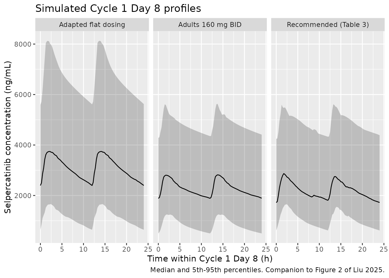
Figures 3 and 4: exposure by age against the adult reference
The paper’s central result is that the Table 3 regimen matches adult exposure across ages 2-17 years (Figure 4), whereas adapted flat dosing overshoots it in younger children (Figure 3, left panels). The next chunk computes the Cycle 1 Day 8 exposures that both figures plot.
adult_ref <- sim_df |>
  dplyr::filter(regimen == "Adults 160 mg BID", time >= 168, time <= 192) |>
  dplyr::group_by(id) |>
  dplyr::summarise(
    cmax = max(Cc),
    auc24 = sum(diff(time) * (head(Cc, -1) + tail(Cc, -1)) / 2),
    .groups = "drop"
  )

adult_target <- c(cmax = median(adult_ref$cmax), auc24 = median(adult_ref$auc24))

peds_exposure <- sim_df |>
  dplyr::filter(regimen != "Adults 160 mg BID", time >= 168, time <= 192) |>
  dplyr::group_by(regimen, id, AGE, WT, BSA, DOSE) |>
  dplyr::summarise(
    cmax = max(Cc),
    auc24 = sum(diff(time) * (head(Cc, -1) + tail(Cc, -1)) / 2),
    .groups = "drop"
  )

# Adult reference level, mg/L and mg*h/L, as plotted in Figures 3 and 4.
c(adult_cmax_mgL = round(adult_target[["cmax"]] / 1000, 2),
  adult_auc24_mghL = round(adult_target[["auc24"]] / 1000, 1))
#>   adult_cmax_mgL adult_auc24_mghL
#>             2.89            53.50
# Replicates Figures 3 and 4 of Liu 2025: simulated Cycle 1 Day 8 Cmax and
# AUC0-24 by age at baseline, with the adult reference level overlaid. Liu 2025
# plots both on the mg/L and mg*h/L scales, followed here.
peds_exposure |>
  tidyr::pivot_longer(c(cmax, auc24), names_to = "metric", values_to = "value") |>
  dplyr::mutate(
    value = value / 1000,
    metric = factor(metric, c("cmax", "auc24"),
                    c("C1D8 Cmax (mg/L)", "C1D8 AUC0-24 (mg*h/L)")),
    reference = ifelse(metric == "C1D8 Cmax (mg/L)",
                       adult_target[["cmax"]] / 1000,
                       adult_target[["auc24"]] / 1000)
  ) |>
  ggplot(aes(AGE, value)) +
  geom_point(alpha = 0.35, size = 0.8) +
  geom_hline(aes(yintercept = reference), colour = "darkorange",
             linetype = "dashed", linewidth = 0.8) +
  geom_smooth(se = FALSE, colour = "steelblue", method = "loess",
              formula = y ~ x) +
  facet_grid(metric ~ regimen, scales = "free_y") +
  labs(x = "Age at baseline (years)", y = NULL,
       title = "Simulated Cycle 1 Day 8 exposure by age",
       caption = paste("Replicates Figures 3 and 4 of Liu 2025.",
                       "Dashed line: simulated adult reference level at 160 mg BID."))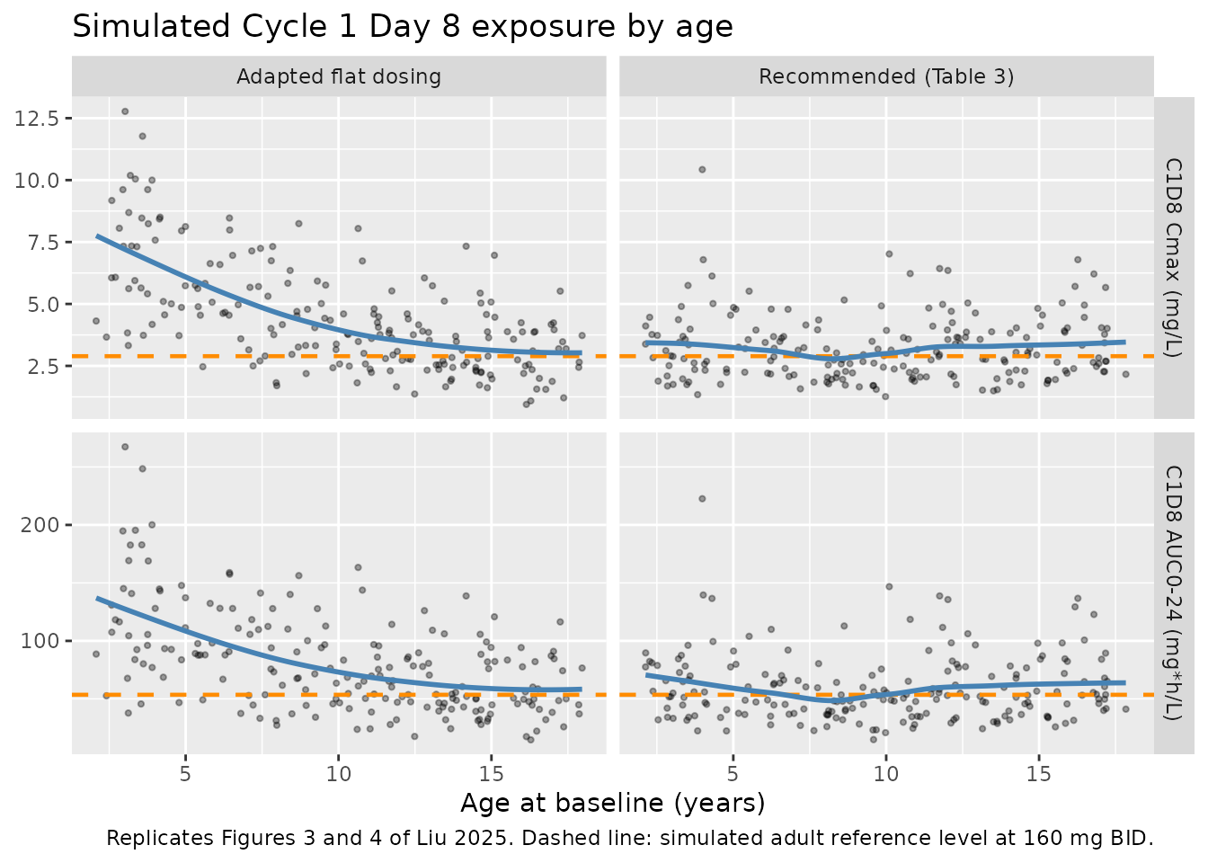
# The paper's conclusion, as an assertion. Both sides are simulated cohorts
# whose spread is driven by which subjects were drawn, so the gates are on the
# CENTRE and on robust quantiles -- never on the extremes.
rec <- dplyr::filter(peds_exposure, regimen == "Recommended (Table 3)")
flat <- dplyr::filter(peds_exposure, regimen == "Adapted flat dosing")

exposure_ratios <- c(
  rec_auc = median(rec$auc24) / adult_target[["auc24"]],
  rec_cmax = median(rec$cmax) / adult_target[["cmax"]],
  flat_auc_under6 = median(flat$auc24[flat$AGE < 6]) / adult_target[["auc24"]],
  rec_auc_under6 = median(rec$auc24[rec$AGE < 6]) / adult_target[["auc24"]]
)
round(exposure_ratios, 3)
#>         rec_auc        rec_cmax flat_auc_under6  rec_auc_under6
#>           0.989           1.015           1.961           1.052

stopifnot(
  # Table 3 regimen matches adult exposure over the whole 2-17 year range.
  abs(exposure_ratios[["rec_auc"]] - 1) < 0.25,
  abs(exposure_ratios[["rec_cmax"]] - 1) < 0.25,
  # Adapted flat dosing overshoots in young children (Figure 3, left panels:
  # "C max and AUC 0-24 values on C1D8 would exceed the exposure observed in
  # adult patients"), and the Table 3 regimen fixes that overshoot.
  exposure_ratios[["flat_auc_under6"]] > 1.5,
  exposure_ratios[["flat_auc_under6"]] > exposure_ratios[["rec_auc_under6"]],
  abs(exposure_ratios[["rec_auc_under6"]] - 1) < 0.35
)
The packaged model reproduces the paper’s conclusion quantitatively: under the Table 3 regimen the median pediatric C1D8 AUC0-24 and Cmax land within a couple of percent of the simulated adult reference, including in the youngest children, while the adapted flat regimen the paper rejected delivers roughly twice the adult AUC0-24 to children under 6 years.
PKNCA validation
NCA is run on Cc rather than on sim,
because the exposures Liu 2025 plots in Figures 3 and 4 are
model-derived simulated values, not observations carrying residual
error; a Cmax taken from sim is upward-biased relative to a
model-derived reference. The interval is the Cycle 1 Day 8 window,
168-192 h, which is where both figures are read.
sim_nca <- sim_df |>
  dplyr::select(id, time, Cc, regimen)

# Guarantee a record at the interval start (168 h) and at time 0 so PKNCA has
# an anchor and does not warn about an AUC range starting before the first
# measurement.
sim_nca <- dplyr::bind_rows(
  sim_nca,
  sim_nca |> dplyr::distinct(id, regimen) |> dplyr::mutate(time = 0, Cc = 0)
) |>
  dplyr::distinct(id, regimen, time, .keep_all = TRUE) |>
  dplyr::arrange(id, regimen, time)

conc_obj <- PKNCA::PKNCAconc(as.data.frame(sim_nca), Cc ~ time | regimen + id)

dose_df <- events |>
  dplyr::filter(evid == 1L) |>
  dplyr::select(id, time, amt, regimen) |>
  as.data.frame()

dose_obj <- PKNCA::PKNCAdose(dose_df, amt ~ time | regimen + id)

intervals <- data.frame(
  start     = 168,
  end       = 192,
  cmax      = TRUE,
  tmax      = TRUE,
  auclast   = TRUE,
  cav       = TRUE,
  half.life = TRUE
)

nca_res <- PKNCA::pk.nca(PKNCA::PKNCAdata(conc_obj, dose_obj,
                                          intervals = intervals))

# `half.life = TRUE` also returns the lambda-z diagnostics PKNCA needs to
# compute it (lambda.z, r.squared, span.ratio, ...); keep only the reported
# parameters. Column selection is by NAME, so the order pivot_wider happens to
# emit is irrelevant.
nca_summary <- as.data.frame(nca_res) |>
  dplyr::filter(PPTESTCD %in% c("cmax", "tmax", "auclast", "cav", "half.life")) |>
  dplyr::group_by(regimen, PPTESTCD) |>
  dplyr::summarise(median = median(PPORRES), .groups = "drop") |>
  tidyr::pivot_wider(names_from = PPTESTCD, values_from = median)

nca_summary |>
  dplyr::select(regimen, cmax, tmax, auclast, cav, half.life) |>
  dplyr::mutate(
    cmax = round(cmax / 1000, 2), auclast = round(auclast / 1000, 1),
    cav = round(cav / 1000, 2), tmax = round(tmax, 2),
    half.life = round(half.life, 1)
  ) |>
  dplyr::rename(
    "Regimen"              = regimen,
    "Cmax (mg/L)"          = cmax,
    "Tmax within C1D8 (h)" = tmax,
    "AUC0-24 (mg*h/L)"     = auclast,
    "Cavg (mg/L)"          = cav,
    "t1/2 (h)"             = half.life
  ) |>
knitr::kable(caption = "PKNCA on the Cycle 1 Day 8 interval (168-192 h), per-subject medians.")| Regimen | Cmax (mg/L) | Tmax within C1D8 (h) | AUC0-24 (mg*h/L) | Cavg (mg/L) | t1/2 (h) |
|---|---|---|---|---|---|
| Adapted flat dosing | 3.88 | 14.00 | 74.9 | 3.12 | 17.3 |
| Adults 160 mg BID | 2.89 | 14.00 | 53.5 | 2.23 | 22.9 |
| Recommended (Table 3) | 2.94 | 14.25 | 53.0 | 2.21 | 15.6 |
Comparison against published exposure
Liu 2025 reports no NCA table. The only published exposure numbers
are the adult reference levels drawn as the orange dashed line in
Figures 3 and 4, which are read off the figures here (roughly 3 mg/L for
C1D8 Cmax and 53 mg*h/L for C1D8 AUC0-24 at 160 mg twice daily). The AUC
reference is independently corroborated by the closed form:
2 * 160 / 6.04 = 53.0 mg*h/L over the two dosing intervals
that make up a day, matching the plotted line to the precision the
figure can be read at.
published <- tibble::tribble(
  ~regimen,               ~cmax,  ~auclast,
  "Adults 160 mg BID",    3000,   53000
)

cmp <- nlmixr2lib::ncaComparisonTable(
  simulated     = nca_res,
  reference     = published,
  by            = "regimen",
  units         = c(cmax = "ng/mL", auclast = "ng*h/mL", tmax = "h",
                    cav = "ng/mL", half.life = "h"),
  tolerance_pct = 20
)

knitr::kable(
  cmp,
  caption = paste("Simulated vs published adult reference exposure.",
                  "* differs from the reference by >20%.",
                  "Reference values are read off the Figure 3 / 4 dashed line."),
  align = c("l", "l", "r", "r", "r")
)| NCA parameter | regimen | Reference | Simulated | % diff |
|---|---|---|---|---|
| Cmax (ng/mL) | Adults 160 mg BID | 3000 | 2890 | -3.6% |
| AUClast (ng*h/mL) | Adults 160 mg BID | 53000 | 53500 | +1.0% |
adult_nca <- as.data.frame(nca_res) |>
  dplyr::filter(regimen == "Adults 160 mg BID") |>
  dplyr::group_by(PPTESTCD) |>
  dplyr::summarise(median = median(PPORRES), .groups = "drop")

adult_med <- setNames(adult_nca$median, adult_nca$PPTESTCD)

# Gate on the CENTRE of the adult arm against the figure-read reference. The
# AUC bound is the tighter of the two because the closed form corroborates the
# reference value; Cmax depends on the absorption parameters and on the drawn
# weight distribution, so it gets the wider envelope.
stopifnot(
  abs(adult_med[["auclast"]] / 53000 - 1) < 0.15,
  abs(adult_med[["cmax"]] / 3000 - 1) < 0.25,
  # Terminal half-life is not published, but must be consistent with a regimen
  # the paper dosed twice daily and describes as at steady state by C1D8.
  adult_med[["half.life"]] > 8, adult_med[["half.life"]] < 60
)
Assumptions and deviations
-
Race distribution. Liu 2025 Table 1 reports sex,
age, weight and BSA but no race breakdown, even though Asian race on F1
is in the final model. All simulated arms are therefore set to
RACE_ASIAN = 0(the reference category), and the covariate’s effect is verified separately as exact algebra in the covariate-regression chunk above (F1 = 1.183 forRACE_ASIAN = 1) rather than by sampling a prevalence that the paper does not publish. - Pediatric age-weight-height mapping. The model reads weight, but the Table 3 dose bands are defined on BSA, so a height is needed to compute Mosteller BSA. Liu 2025 sampled covariates from the NHANES DXA database, which is not reproduced here. Instead age is drawn uniformly over 2-18 years (to cover the Figure 4 x-axis evenly) and weight and height are read off 50th-percentile paediatric growth references, with the weight curve rescaled by a single factor so that it passes through the paper’s own LIBRETTO-121 median pair (14.0 years, 48.5 kg; Table 1). The resulting median BSA at that age reproduces the reported 1.47 m^2 to within 0.05 m^2, which is asserted above. Weight carries 15% and height 4% lognormal scatter.
- Adult weight distribution. Drawn lognormal to the LIBRETTO-001 median of 67.3 kg with the Table 1 spread, truncated to the observed 26.8-179 kg range. The paper’s adult reference line comes from NHANES adults instead, whose weight distribution is heavier; this is the main reason the simulated adult Cmax sits slightly below the figure-read 3 mg/L.
-
Dose covariate.
DOSEis set equal to the per-administration amount on every record and held constant, i.e. no dose reductions or escalations are simulated. Liu 2025 modelledDOSEas time-varying precisely to absorb the reductions that occurred in the trials, but it does not publish the reduction pattern, so a constant dose per subject is the only reproducible choice. - 40 mg three times a day is simulated as every 8 hours. Table 3 says “TID” without specifying the clock times.
- Cycle 1 Day 8 window. Taken as 168-192 h with the first dose at time 0 (i.e. Day 1 spans 0-24 h). Figures 3 and 4 report “Cycle 1 Day 8” exposures without stating the exact window.
- AUC0-24 covers two dosing intervals, as Liu 2025 defines it (“area under the curve over two dosing intervals (AUC0-24)”). For the 40 mg three-times-a- day arm the same 24 h window contains three doses; the paper plots that arm on the same AUC0-24 axis, so the window and not the dose count is what is held fixed.
-
No parameter came from outside the paper. Every
ini()value is from Liu 2025 Table 2. No author correspondence, no upstream model, no figure digitisation for any parameter value. The only digitised numbers anywhere in this vignette are the two adult reference levels (3 mg/L and 53 mg*h/L) read off the Figure 3 / 4 dashed line, which are validation targets and feed no parameter. - No maturation term. The model has none, and the paper is explicit that predictions below 2 years of age may overpredict concentrations because CYP3A4, selpercatinib’s main metabolic route, matures around 2 years and no patient under 2 years was in the dataset. Simulations here start at 2 years, matching the approved age range.
Errata and internal discrepancies in the source
- The additive residual error’s unit tag is wrong. Table 2 prints “Additive RUV (mg/L) 61.5”, but 61.5 mg/L cannot be a concentration standard deviation for this model: Figure 3 puts the adult C1D8 Cmax at 160 mg twice daily near 3 mg/L, so the tag would make the additive error roughly twenty times the peak concentration. The value is on the analysis-dataset scale of ng/mL, which Figure 2 states on its y-axis (“Prediction-corrected selpercatinib concentrations (ng/mL)”, data spanning about 1000-10000 ng/mL) and which matches the 1 ng/mL assay limit of quantification. 61.5 ng/mL is 2.5% of the roughly 2500 ng/mL median steady-state concentration. The model file is written on the ng/mL scale so that the Table 2 number is used verbatim.
- Two concentration scales coexist in the paper. Figure 2 (the pcVPC, i.e. the fitting scale) is in ng/mL while Figures 3 and 4 (the simulated exposures) are in mg/L and mg*h/L. Both are used above: the model observes in ng/mL and the figure replications divide by 1000.
-
The IIV convention is not stated. Table 2’s IIV
column gives percentages with no footnote saying whether they are
sqrt(exp(omega^2) - 1) * 100oromega * 100, and the column carries no confidence interval that could settle it by variance symmetry. The log-normal readingomega^2 = log(CV^2 + 1)is used here. Under the alternativeomega = CVreading the standard deviations would be larger by 6% (CL/F 0.488 vs 0.462), 10% (Vc/F 0.661 vs 0.602), 9% (ka 0.636 vs 0.583) and 7% (Dur 0.562 vs 0.524). None of the assertions above is sensitive to the choice, because all of them are on medians, on typical-value algebra, or on ratios between two arms that share the same omegas. - Both residual terms are read as standard deviations, not variances. Table 2 tags them with linear scales – a concentration unit for the additive term and “fraction” for the proportional one, where a variance would carry squared units – and the same table reports IIV as CV%, i.e. on the standard-deviation scale throughout. Under a variance reading the proportional error would be 50.3% rather than 25.3% and the additive term negligible.
-
The Table 2 dose effect on CL/F is linear and does not
extrapolate. The multiplier
1 - 0.00321 * (DOSE - 160)reaches zero at 471.5 mg and turns negative above it. No clamp is imposed in the model file because the paper imposes none; keepDOSEinside the 20-240 mg range the model was fit to. -
A statistically significant age effect on CL/F was
deliberately excluded. Automated stepwise covariate modelling
retained age on CL/F after backward deletion (p < 0.001), and the
Discussion reports that adding it dropped the objective function by
43.998 points as a linear model centred on the median age of 58 years
and by 49.995 points as a segmented “hockey stick” model with the break
point at the same age. Both, however, “resulted in biased population
predictions in children” and underpredicted the C1D8 profiles in
LIBRETTO-121, so the effect was removed during model refinement. Neither
coefficient is published, so neither is encodable; the excluded
covariate is documented in the model file’s
covariatesDataExcluded$AGE. - Figure 1’s caption is garbled in the typeset article. The caption text reads “Schematic view of the final population is the covariate associated pharmacokinetic model. Note: Text in italics with the adjacent pharmacokinetic parameter”, i.e. two sentences interleaved. The intended reading, recoverable from the layout, is “Schematic view of the final population pharmacokinetic model. Note: Text in italics is the covariate associated with the adjacent pharmacokinetic parameter.” The schematic itself is unambiguous.
- Table 1’s BSA range is printed without a separator (“0.4462.79” in the Total column), which is 0.446-2.79 as the study columns show.
- Table S1 double-counts a CYP3A4 inducer row. The strong and moderate CYP3A4 inducer rows each report 3 (0.4%) patients in LIBRETTO-001 and 0 in LIBRETTO-121, yet both give a Total of 6 (0.4%). The “Any CYP3A4 inducers” row (6 patients) is the consistent one. This affects no model parameter – concomitant medication was screened and not retained.