Ticagrelor during VA-ECMO (Kang 2026)
Source:vignettes/articles/Kang_2026_ticagrelor.Rmd
Kang_2026_ticagrelor.RmdModel and source
- Citation: Kang S, Min KL, Yang S, Hahn J, Kim D, Jin BH, Chae SU, Bae SK, Wi J, Chang MJ. Population Pharmacokinetics of Ticagrelor during Veno-Arterial ECMO in Acute Coronary Syndrome: Model-Informed Dosing Simulations. Clin Pharmacol Ther. 2026;120(1):193-202. doi:10.1002/cpt.70282
- Description: Joint parent-metabolite one-compartment population PK model for ticagrelor and its active metabolite AR-C124910XX (TAM) in adults with acute coronary syndrome supported by veno-arterial extracorporeal membrane oxygenation (VA-ECMO) (Kang 2026). First-order absorption from a depot into the ticagrelor central compartment; ticagrelor leaves the central compartment by two parallel first-order routes sharing the same apparent clearance CL/F - a non-metabolic route (fraction 1 - fm) and a metabolic route (fraction fm) that forms TAM in its own one-compartment space with its own apparent clearance CLM/F and volume VM/F. Ka and fm were fixed for identifiability, and both additive residual error terms were fixed to preliminary estimates. Final-model covariates: a binary ECMO treatment-status indicator reducing CL/F 0.35-fold and expanding Vd/F 2.74-fold, plus an ECMO circuit blood-flow power term 0.518^(Q_ECMO/3) on Vd/F that applies only while on ECMO.
- Article: https://doi.org/10.1002/cpt.70282
- Supplement (Figures S1-S4, Table S1, Appendices S1-S3, including the NONMEM control file): https://europepmc.org/article/PMC/PMC13264463
Kang 2026 is the first clinical study of ticagrelor and its active metabolite AR-C124910XX (TAM) in patients supported by veno-arterial extracorporeal membrane oxygenation (VA-ECMO), and the first ticagrelor model to fit parent and metabolite jointly rather than as two separate models.
Units. The model works in mg, L and hours, so
concentrations are in mg/L. The paper reports
concentrations in ng/mL, including its 180-360 ng/mL target window. This
vignette converts with * 1000 wherever it compares against
the paper; the conversion is explained in the Errata.
Population
Twenty adults with acute coronary syndrome (19 STEMI, 1 NSTEMI; 19 underwent PCI; 15 had cardiac arrest) were enrolled prospectively in the coronary intensive care unit of Severance Hospital, Seoul, between October 2015 and April 2018 (Kang 2026 Table 1). Median age was 59 years (range 36-88), median body weight 70.2 kg (58-110), median BMI 25.1 kg/m^2 (20.7-35.9); 18 of 20 were men. All patients were transfused, 18 received albumin, and the median VA-ECMO duration was 5.87 days (1.82-16.26).
The cohort was critically ill on both occasions: median serum creatinine was 1.30 mg/dL on ECMO versus 1.72 mg/dL after weaning, median BUN 20.8 versus 43.8 mg/dL, median albumin 2.9 versus 2.95 g/dL and median total protein 4.9 versus 5.55 g/dL. Five patients received CRRT while on ECMO and six after weaning.
All patients received the standard ACS regimen – a 180 mg ticagrelor loading dose followed by 90 mg twice daily. Paired sampling at pre-dose and 1, 2, 3, 6, 8 and 12 h was planned during ECMO (at least 24 h after initiation) and again after weaning, yielding 225 ticagrelor and 225 AR-C124910XX concentrations (127 ON-ECMO from 19 patients, 98 OFF-ECMO from 13 patients). The reduced 45-135 mg regimens discussed in the paper are simulated, never observed.
The same information is available programmatically via
readModelDb("Kang_2026_ticagrelor")()$population.
Source trace
Per-parameter provenance is recorded as an in-file comment beside
each ini() entry in
inst/modeldb/specificDrugs/Kang_2026_ticagrelor.R. The
table collects them in one place.
| Equation / parameter | Value | Source location |
|---|---|---|
lcl (CL/F, OFF-ECMO) |
12.2 L/h | Table 2, theta CL/F (RSE 16.7%; bootstrap
8.99-16.24) |
lvc (Vd/F, OFF-ECMO) |
157 L | Table 2, theta Vd/F (RSE 17.4%; bootstrap
101.04-291.14) |
lcl_tam (CLM/F) |
8.8 L/h | Table 2, theta CLM/F (RSE 10.7%; bootstrap
7.27-10.76) |
lvc_tam (VM/F) |
29.5 L | Table 2, theta VM/F (RSE 42.7%; bootstrap
12.63-102.22) |
lka (Ka) |
0.533 1/h, FIXED | Table 2, theta Ka = “0.533 FIX”; Methods, “Population
PK modeling” |
fm (FMET) |
0.224, FIXED | Table 2, theta FMET = “0.224 FIX”; fixed from refs
23-24 (non-ECMO models) |
e_ecmo_cl |
0.35 | Table 2, theta ECMO on CL/F (RSE 6.5%; bootstrap
0.302-0.433) |
e_ecmo_vc |
2.74 | Table 2, theta ECMO on Vd/F (RSE 34.5%; bootstrap
1.28-5.30) |
e_qecmo_vc |
0.518 | Table 2, theta ECMO flow rate on Vd/F (RSE 32%;
bootstrap 0.248-0.839) |
etalcl |
0.441 (74.4% CV) | Table 2, omega^2 CL/F; footnote b gives %CV =
sqrt(exp(w^2)-1)*100 |
etalvc |
0.661 (96.8% CV) | Table 2, omega^2 Vd/F
|
etalcl_tam |
0.156 (41.1% CV) | Table 2, omega^2 CLM/F
|
addSd |
1.65 * sqrt(0.1) = 0.5218 mg/L, FIXED | Table 2, sigma ADD = “1.65 FIX”; footnote c, residual
SD = sqrt(0.1) x W |
addSd_tam |
0.2 * sqrt(0.1) = 0.06325 mg/L, FIXED | Table 2, sigma ADDM = “0.2 FIX”; footnote c |
CL/F = 12.2 * 0.35^ECMO |
n/a | Results, “Population PK modeling and evaluation”; Appendix S1;
Appendix S2 $PK
|
Vd/F = 157 * 2.74^ECMO * (0.518^(flow/3))^ECMO |
n/a | Appendix S2 $PK (control stream); main-text form in
Results (see Errata) |
k20 = (1-fm)*CL/Vd, k23 = fm*CL/Vd,
k30 = CLM/VM
|
n/a | Figure 1 caption; Appendix S1, “The elimination rate constants were defined as” |
d/dt system (depot -> central ->
central_tam) |
n/a | Appendix S1 differential equations; Appendix S2
$DES
|
Cc = central/Vd,
Cc_tam = central_tam/VM
|
n/a | Appendix S1 (S2 = Vd/F, S3 = VM/F);
Appendix S2 $ERROR
|
| Additive error on both analytes | n/a | Methods, “Statistical analysis”/“Population PK modeling”; Appendix
S2 $ERROR Y = IPRED + W*EPS(1)
|
Structural verification
Every derived quantity the paper prints in prose is pure algebra on
the ini() values, so it can be reproduced exactly. These
gates are deterministic – they carry no simulation noise and are
therefore asserted tightly.
mod <- readModelDb("Kang_2026_ticagrelor")
ui  <- rxode2::rxode(mod)
#> ℹ parameter labels from comments will be replaced by 'label()'
th  <- ui$theta

cl_off <- exp(th[["lcl"]])
vc_off <- exp(th[["lvc"]])
e_cl   <- th[["e_ecmo_cl"]]
e_vc   <- th[["e_ecmo_vc"]]
e_q    <- th[["e_qecmo_vc"]]

# Vd/F on ECMO at an arbitrary circuit flow (L/min).
vd_on <- function(flow) vc_off * e_vc * e_q^(flow / 3)

printed <- tibble::tribble(
  ~quantity,                            ~published, ~reproduced,
  "CL/F OFF-ECMO (L/h)",                12.2,       cl_off,
  "CL/F ON-ECMO (L/h)",                 4.27,       cl_off * e_cl,
  "Vd/F ON-ECMO at 3 L/min (L)",        222.8,      vd_on(3),
  "Vd/F ON-ECMO at 1 L/min (L)",        345.5,      vd_on(1),
  "Vd/F 'OFF-ECMO' at 3 L/min (L)",     81.3,       vd_on(3) / e_vc,
  "IIV CL/F (%CV)",                     74.4,       100 * sqrt(exp(0.441) - 1),
  "IIV Vd/F (%CV)",                     96.8,       100 * sqrt(exp(0.661) - 1),
  "IIV CLM/F (%CV)",                    41.1,       100 * sqrt(exp(0.156) - 1)
) |>
  dplyr::mutate(pct_diff = 100 * (reproduced - published) / published)

printed |>
  dplyr::rename(
    "Quantity"          = quantity,
    "Published"         = published,
    "Reproduced"        = reproduced,
    "Difference (%)"    = pct_diff
  ) |>
  knitr::kable(digits = c(0, 2, 3, 3),
caption = "Published derived quantities reproduced from the packaged ini() values.")| Quantity | Published | Reproduced | Difference (%) |
|---|---|---|---|
| CL/F OFF-ECMO (L/h) | 12.20 | 12.200 | 0.000 |
| CL/F ON-ECMO (L/h) | 4.27 | 4.270 | 0.000 |
| Vd/F ON-ECMO at 3 L/min (L) | 222.80 | 222.833 | 0.015 |
| Vd/F ON-ECMO at 1 L/min (L) | 345.50 | 345.483 | -0.005 |
| Vd/F ‘OFF-ECMO’ at 3 L/min (L) | 81.30 | 81.326 | 0.032 |
| IIV CL/F (%CV) | 74.40 | 74.449 | 0.065 |
| IIV Vd/F (%CV) | 96.80 | 96.785 | -0.016 |
| IIV CLM/F (%CV) | 41.10 | 41.088 | -0.028 |
# Exact algebra: every row must agree to better than 0.1%.
stopifnot(all(abs(printed$pct_diff) < 0.1))

# The ODE system must NOT have been silently replaced by an analytic solution.
stopifnot(is.null(ui$linCmt), identical(ui$state, c("depot", "central", "central_tam")))
The 81.3 L the paper labels “OFF-ECMO” is the
222.8 L ON-ECMO value divided by the 2.74-fold ECMO effect
at the same 3 L/min flow – a matched-flow counterfactual that isolates
the volume expansion, not a value the model produces for a decannulated
patient (see Errata).
Single-dose typical profile and PKNCA validation
The strongest available gate is closed-form: for this structure the
parent’s total apparent clearance is CL/F regardless of how
the flux splits between the non-metabolic (k20) and
metabolic (k23) routes, so
CL/F * AUCinf = Dose exactly. Likewise exactly
fm of the dose reaches TAM, so
CLM/F * AUCinf_TAM = fm * Dose. Both identities are
independent of the covariate values, which makes them a free regression
test on the whole ODE system.
mod_typ <- rxode2::zeroRe(mod)
#> ℹ parameter labels from comments will be replaced by 'label()'

# Route A event table (cmt = ODE state + explicit dvid): this model declares two
# endpoints, so every observation row must nominate one. rxSolve still returns
# both Cc and Cc_tam as columns.
make_single <- function(regimen, ecmo, flow, dose = 180, tmax = 336, id = 1L) {
  tg <- sort(unique(c(seq(0, tmax, by = 0.25), 0)))
  dplyr::bind_rows(
    tibble::tibble(id = id, time = 0,  amt = dose,      cmt = "depot",
                   evid = 1L, dvid = NA_integer_),
    tibble::tibble(id = id, time = tg, amt = NA_real_,  cmt = "central",
                   evid = 0L, dvid = 1L)
  ) |>
    dplyr::mutate(regimen = regimen, ECMO_STATUS = ecmo, Q_ECMO = flow) |>
    dplyr::arrange(time, dplyr::desc(evid))
}

single_events <- dplyr::bind_rows(
  make_single("OFF-ECMO",            ecmo = 0L, flow = 0,   id = 1L),
  make_single("ON-ECMO, 3.0 L/min",  ecmo = 1L, flow = 3,   id = 2L),
  make_single("ON-ECMO, 1.0 L/min",  ecmo = 1L, flow = 1,   id = 3L)
)

sim_single <- rxode2::rxSolve(
  mod_typ, events = single_events,
  keep = c("regimen"), covsInterpolation = "locf",
  returnType = "data.frame"
)
#> ℹ omega/sigma items treated as zero: 'etalcl', 'etalvc', 'etalcl_tam'
#> Warning: multi-subject simulation without without 'omega'
sim_single |>
  dplyr::select(time, regimen, Ticagrelor = Cc, `AR-C124910XX` = Cc_tam) |>
  tidyr::pivot_longer(c(Ticagrelor, `AR-C124910XX`),
                      names_to = "analyte", values_to = "conc") |>
  dplyr::filter(time > 0, time <= 168) |>
  ggplot(aes(time, conc * 1000, colour = regimen)) +
  geom_line() +
  facet_wrap(~analyte, scales = "free_y") +
  scale_x_continuous(breaks = seq(0, 168, by = 24)) +
  scale_y_log10() +
  labs(x = "Time (h)", y = "Concentration (ng/mL)", colour = NULL,
       title = "Typical-value profiles after a single 180 mg loading dose",
       caption = paste("VA-ECMO lowers CL/F 2.9-fold and raises Vd/F, so parent",
                       "exposure rises and the terminal phase lengthens;",
                       "metabolite exposure is unchanged.")) +
  theme(legend.position = "bottom")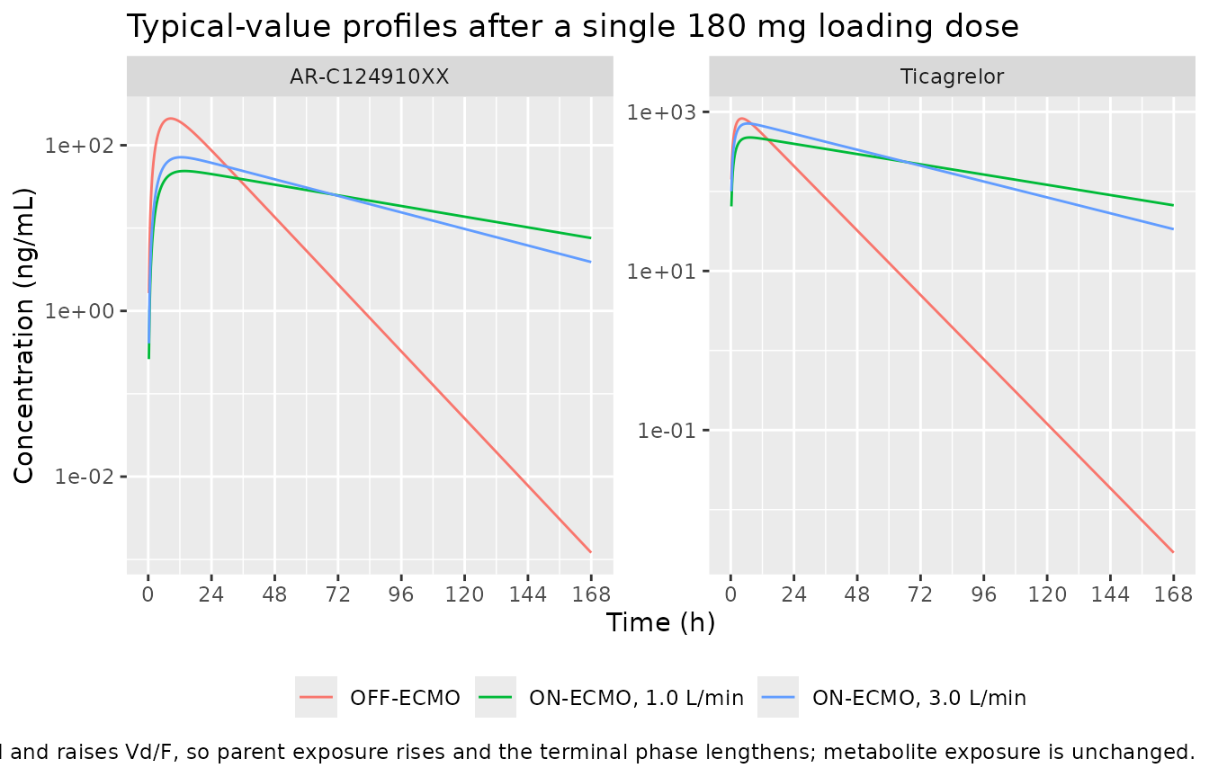
# PKNCA input: filter on !is.na() only -- a `time > 0` or `Cc > 0` filter would
# drop the time-zero anchor and trigger the "AUC range starting (0) before the
# first measurement" warning for every subject.
conc_parent <- sim_single |>
  dplyr::filter(!is.na(Cc)) |>
  dplyr::select(id, time, regimen, Cc)

conc_parent <- dplyr::bind_rows(
  conc_parent,
  conc_parent |> dplyr::distinct(id, regimen) |> dplyr::mutate(time = 0, Cc = 0)
) |>
  dplyr::distinct(id, regimen, time, .keep_all = TRUE) |>
  dplyr::arrange(id, regimen, time)

dose_df <- single_events |>
  dplyr::filter(evid == 1) |>
  dplyr::select(id, time, amt, regimen)

intervals <- data.frame(start = 0, end = Inf,
                        cmax = TRUE, tmax = TRUE,
                        aucinf.obs = TRUE, half.life = TRUE)

nca_parent <- PKNCA::pk.nca(PKNCA::PKNCAdata(
  PKNCA::PKNCAconc(conc_parent, Cc ~ time | regimen + id),
  PKNCA::PKNCAdose(dose_df,     amt ~ time | regimen + id),
  intervals = intervals
))
conc_tam <- sim_single |>
  dplyr::filter(!is.na(Cc_tam)) |>
  dplyr::select(id, time, regimen, Cc_tam)

conc_tam <- dplyr::bind_rows(
  conc_tam,
  conc_tam |> dplyr::distinct(id, regimen) |> dplyr::mutate(time = 0, Cc_tam = 0)
) |>
  dplyr::distinct(id, regimen, time, .keep_all = TRUE) |>
  dplyr::arrange(id, regimen, time)

nca_tam <- PKNCA::pk.nca(PKNCA::PKNCAdata(
  PKNCA::PKNCAconc(conc_tam, Cc_tam ~ time | regimen + id),
  PKNCA::PKNCAdose(dose_df,  amt    ~ time | regimen + id),
  intervals = intervals
))
tidy_nca <- function(res, analyte) {
  as.data.frame(res) |>
    dplyr::filter(PPTESTCD %in% c("cmax", "tmax", "aucinf.obs", "half.life")) |>
    dplyr::mutate(analyte = analyte) |>
    dplyr::select(analyte, regimen, PPTESTCD, PPORRES)
}

nca_all <- dplyr::bind_rows(
  tidy_nca(nca_parent, "Ticagrelor"),
  tidy_nca(nca_tam,    "AR-C124910XX")
) |>
  tidyr::pivot_wider(names_from = PPTESTCD, values_from = PPORRES)

nca_all |>
  dplyr::mutate(
    cmax       = cmax * 1000,
    aucinf.obs = aucinf.obs * 1000
  ) |>
  dplyr::select(analyte, regimen, cmax, tmax, aucinf.obs, half.life) |>
  dplyr::rename(
    "Analyte"            = analyte,
    "Scenario"           = regimen,
    "Cmax (ng/mL)"       = cmax,
    "Tmax (h)"           = tmax,
    "AUCinf (ng*h/mL)"   = aucinf.obs,
    "t1/2 (h)"           = half.life
  ) |>
  knitr::kable(digits = 1,
caption = "PKNCA on the typical-value single-180-mg-dose profiles.")| Analyte | Scenario | Cmax (ng/mL) | Tmax (h) | AUCinf (ng*h/mL) | t1/2 (h) |
|---|---|---|---|---|---|
| Ticagrelor | OFF-ECMO | 825.4 | 4.2 | 14750.6 | 8.9 |
| Ticagrelor | ON-ECMO, 1.0 L/min | 476.5 | 7.2 | 42153.2 | 56.1 |
| Ticagrelor | ON-ECMO, 3.0 L/min | 713.6 | 6.5 | 42152.3 | 36.2 |
| AR-C124910XX | OFF-ECMO | 210.3 | 8.5 | 4581.7 | 8.9 |
| AR-C124910XX | ON-ECMO, 1.0 L/min | 48.9 | 13.8 | 4581.9 | 56.1 |
| AR-C124910XX | ON-ECMO, 3.0 L/min | 71.6 | 12.5 | 4581.8 | 36.2 |
gate <- nca_all |>
  dplyr::left_join(
    dplyr::distinct(single_events[single_events$evid == 1, c("regimen", "ECMO_STATUS", "Q_ECMO")]),
    by = "regimen"
  ) |>
  dplyr::mutate(
    cl_expect = dplyr::if_else(analyte == "Ticagrelor",
                               cl_off * e_cl^ECMO_STATUS,
                               exp(th[["lcl_tam"]])),
    dose_in   = dplyr::if_else(analyte == "Ticagrelor", 180, 0.224 * 180),
    # Closed-form identity: clearance x AUCinf must recover the amount entering
    # that compartment. Exact for both analytes, for every covariate setting.
    balance   = cl_expect * aucinf.obs / dose_in
  )

gate |>
  dplyr::select(analyte, regimen, balance) |>
  dplyr::rename("Analyte" = analyte, "Scenario" = regimen,
                "CL x AUCinf / amount in" = balance) |>
  knitr::kable(digits = 4,
caption = "Mass-balance gate. Every entry must be 1.")| Analyte | Scenario | CL x AUCinf / amount in |
|---|---|---|
| Ticagrelor | OFF-ECMO | 0.9998 |
| Ticagrelor | ON-ECMO, 1.0 L/min | 1.0000 |
| Ticagrelor | ON-ECMO, 3.0 L/min | 0.9999 |
| AR-C124910XX | OFF-ECMO | 1.0000 |
| AR-C124910XX | ON-ECMO, 1.0 L/min | 1.0000 |
| AR-C124910XX | ON-ECMO, 3.0 L/min | 1.0000 |
# Numerical-integration error only; this is a solve against its own closed form,
# so the bound is tight on purpose.
stopifnot(all(abs(gate$balance - 1) < 0.005))

# Parent terminal half-life is ln(2) * Vd / CL (ka = 0.533 /h is far faster than
# either elimination rate, so there is no flip-flop).
hl_parent <- nca_all |> dplyr::filter(analyte == "Ticagrelor")
hl_expect <- c("OFF-ECMO"           = log(2) * vc_off  / cl_off,
               "ON-ECMO, 3.0 L/min" = log(2) * vd_on(3) / (cl_off * e_cl),
               "ON-ECMO, 1.0 L/min" = log(2) * vd_on(1) / (cl_off * e_cl))
stopifnot(all(abs(hl_parent$half.life /
                    hl_expect[hl_parent$regimen] - 1) < 0.02))

# The metabolite is formation-rate limited: k30 = CLM/VM = 0.298 /h is an order
# of magnitude faster than the parent's elimination, so the TAM terminal slope
# returns the PARENT half-life, not ln(2)/k30 = 2.3 h.
hl_tam <- nca_all |> dplyr::filter(analyte == "AR-C124910XX")
stopifnot(
  all(abs(hl_tam$half.life / hl_expect[hl_tam$regimen] - 1) < 0.05),
  log(2) / (exp(th[["lcl_tam"]]) / exp(th[["lvc_tam"]])) < 3
)
Metabolite-to-parent exposure ratio
The model has a closed form for this too:
AUC_TAM / AUC_parent = fm * CL / CLM, which depends on ECMO
status only through CL.
ratio <- nca_all |>
  dplyr::select(analyte, regimen, aucinf.obs) |>
  tidyr::pivot_wider(names_from = analyte, values_from = aucinf.obs) |>
  dplyr::mutate(
    observed = `AR-C124910XX` / Ticagrelor,
    closed_form = 0.224 * c(cl_off, cl_off * e_cl, cl_off * e_cl) / exp(th[["lcl_tam"]])
  )

ratio |>
  dplyr::mutate(dplyr::across(c(observed, closed_form), ~ 100 * .x)) |>
  dplyr::select(regimen, observed, closed_form) |>
  dplyr::rename("Scenario" = regimen,
                "Simulated AUC ratio (%)" = observed,
                "fm * CL / CLM (%)"       = closed_form) |>
  knitr::kable(digits = 1,
caption = "TAM:ticagrelor AUCinf ratio versus its closed form.")| Scenario | Simulated AUC ratio (%) | fm * CL / CLM (%) |
|---|---|---|
| OFF-ECMO | 31.1 | 31.1 |
| ON-ECMO, 1.0 L/min | 10.9 | 10.9 |
| ON-ECMO, 3.0 L/min | 10.9 | 10.9 |
stopifnot(all(abs(ratio$observed / ratio$closed_form - 1) < 0.01))

# External consistency: the paper's Introduction states AR-C124910XX
# "constitutes ~30-40% of the concentration of ticagrelor exposure" in non-ECMO
# populations. The OFF-ECMO arm should land in that window.
off_ratio <- 100 * ratio$observed[ratio$regimen == "OFF-ECMO"]
stopifnot(off_ratio > 25, off_ratio < 45)
The ON-ECMO ratio falls to about 11% because VA-ECMO nearly triples
parent exposure while leaving metabolite exposure untouched –
fm and CLM/F carry no ECMO effect, so the
amount of TAM formed per dose is invariant. This is a direct structural
consequence of the published model rather than an observation, and it is
a concrete prediction the paper does not itself state.
Virtual cohort: ON-ECMO versus OFF-ECMO at the observed regimen
The trial’s actual regimen was 180 mg then 90 mg twice daily. Two 200-subject arms are simulated at that regimen – one on ECMO at the 3.4 L/min flow used in the paper’s own scenarios, one after weaning.
set.seed(20260914)
rxode2::rxSetSeed(20260914)

make_cohort <- function(n, arm, ecmo, flow, id_offset = 0L,
                        ld = 180, md = 90, tau = 12, tend = 168) {
  dose_t <- c(0, seq(tau, tend, by = tau))
  amts   <- c(ld, rep(md, length(dose_t) - 1L))
  obs_t  <- seq(0, tend, by = 1)
  ids    <- id_offset + seq_len(n)
  dplyr::bind_rows(
    tidyr::expand_grid(id = ids, idx = seq_along(dose_t)) |>
      dplyr::mutate(time = dose_t[idx], amt = amts[idx], cmt = "depot",
                    evid = 1L, dvid = NA_integer_) |>
      dplyr::select(-idx),
    tidyr::expand_grid(id = ids, time = obs_t) |>
      dplyr::mutate(amt = NA_real_, cmt = "central", evid = 0L, dvid = 1L)
  ) |>
    dplyr::mutate(arm = arm, ECMO_STATUS = ecmo, Q_ECMO = flow) |>
    dplyr::arrange(id, time, dplyr::desc(evid))
}

cohort_events <- dplyr::bind_rows(
  make_cohort(200, "ON-ECMO (3.4 L/min)",  ecmo = 1L, flow = 3.4, id_offset =   0L),
  make_cohort(200, "OFF-ECMO",             ecmo = 0L, flow = 0,   id_offset = 200L)
)

# Disjoint IDs are mandatory: duplicate ids across arms silently merge subjects.
stopifnot(!anyDuplicated(unique(cohort_events[, c("id", "time", "evid")])))

sim_cohort <- rxode2::rxSolve(
  mod, events = cohort_events, keep = c("arm"),
  covsInterpolation = "locf", returnType = "data.frame"
)
#> ℹ parameter labels from comments will be replaced by 'label()'
sim_cohort |>
  dplyr::filter(time > 0) |>
  dplyr::group_by(arm, time) |>
  dplyr::summarise(
    p10 = quantile(Cc, 0.10), p50 = median(Cc), p90 = quantile(Cc, 0.90),
    .groups = "drop"
  ) |>
  ggplot(aes(time, p50 * 1000)) +
  geom_ribbon(aes(ymin = p10 * 1000, ymax = p90 * 1000), alpha = 0.2) +
  geom_line() +
  geom_hline(yintercept = c(180, 360), linetype = "dashed", colour = "grey40") +
  facet_wrap(~arm) +
  scale_x_continuous(breaks = seq(0, 168, by = 24)) +
  scale_y_log10() +
  labs(x = "Time (h)", y = "Ticagrelor (ng/mL)",
       title = "Standard 180 mg / 90 mg q12h regimen, ON- versus OFF-ECMO",
       caption = paste("Median and 10th-90th percentiles, 200 subjects per arm.",
                       "Dashed lines are the paper's 180-360 ng/mL target window."))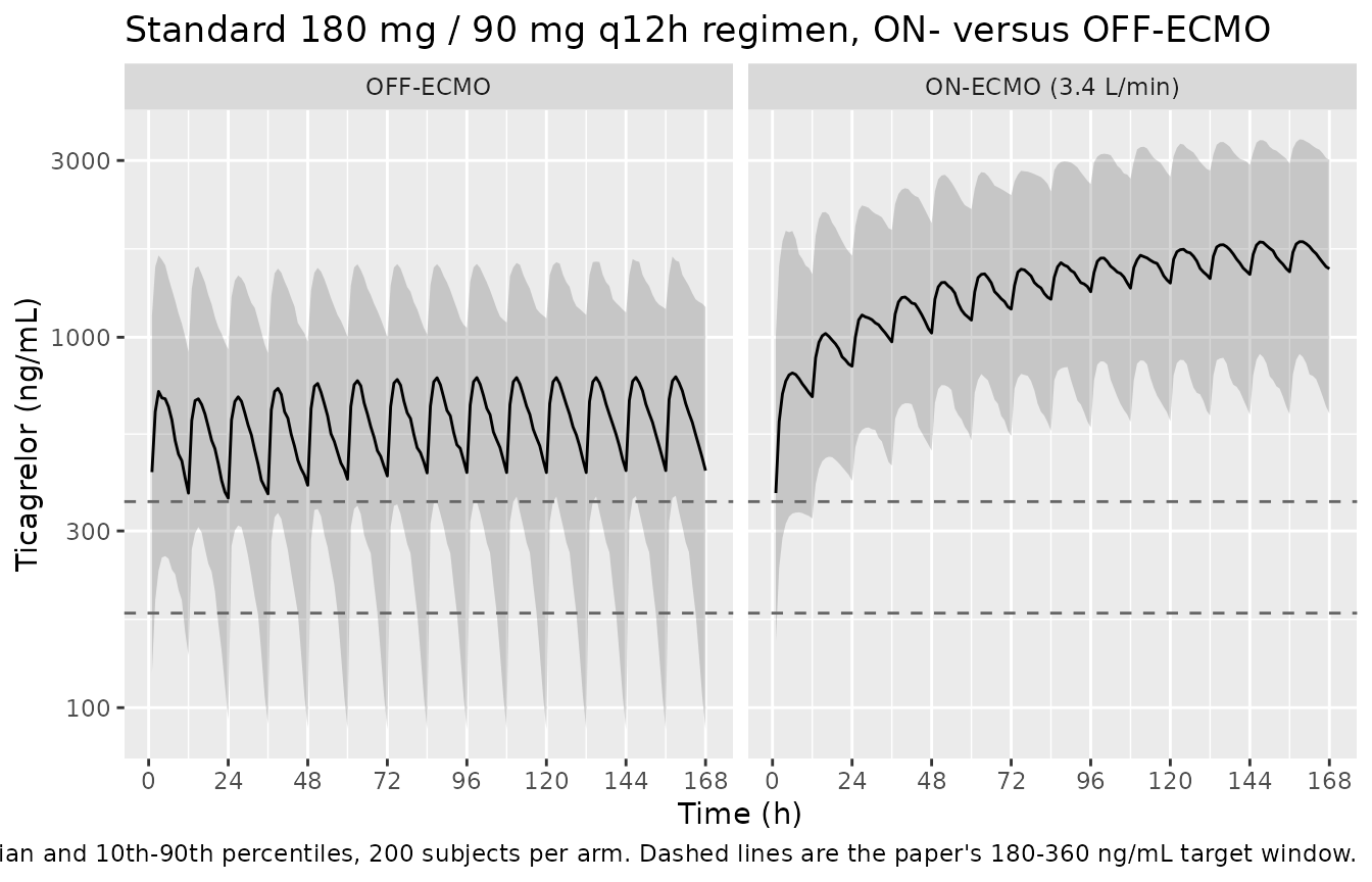
# Steady-state trough on the standard regimen, at the end of the last complete
# interval. Assertions are on the MEDIAN and a robust quantile, never on the
# cohort extremes, which are not reproducible across rxode2 builds or thread
# counts.
trough <- sim_cohort |>
  dplyr::filter(time == 168) |>
  dplyr::group_by(arm) |>
  dplyr::summarise(
    median_ng = median(Cc) * 1000,
    q25_ng    = quantile(Cc, 0.25) * 1000,
    q75_ng    = quantile(Cc, 0.75) * 1000,
    pct_above_360 = 100 * mean(Cc * 1000 > 360),
    .groups = "drop"
  )

trough |>
  dplyr::rename(
    "Arm"                      = arm,
    "Median trough (ng/mL)"    = median_ng,
    "Q1 (ng/mL)"               = q25_ng,
    "Q3 (ng/mL)"               = q75_ng,
    "Above 360 ng/mL (%)"      = pct_above_360
  ) |>
  knitr::kable(digits = 1,
caption = "Simulated 168 h trough on the standard 90 mg q12h regimen.")| Arm | Median trough (ng/mL) | Q1 (ng/mL) | Q3 (ng/mL) | Above 360 ng/mL (%) |
|---|---|---|---|---|
| OFF-ECMO | 436.5 | 208.2 | 713.5 | 57.0 |
| ON-ECMO (3.4 L/min) | 1530.2 | 1019.2 | 2168.1 | 97.5 |
on  <- trough[trough$arm == "ON-ECMO (3.4 L/min)", ]
off <- trough[trough$arm == "OFF-ECMO", ]

# The paper's central claim is that VA-ECMO raises exposure enough that standard
# dosing overshoots. Gate on the ratio of medians, which is driven by the 1/0.35
# clearance effect (2.86-fold) and is therefore a structural quantity, not a
# tail statistic.
stopifnot(
  on$median_ng / off$median_ng > 2,
  on$median_ng / off$median_ng < 4,
  # Standard dosing on ECMO puts the typical patient well above the upper bound.
  on$median_ng > 360,
  # ... and a clear majority of the ON-ECMO arm with it.
  on$pct_above_360 > 60
)
Replicating Figure 3: the 6-day ECMO weaning plan
Kang 2026 Figure 3 simulates a 6-day plan – circuit flow held at 3.4 L/min for 3 days, reduced 0.3 L/min every 6 h over the next 2 days, held at 1 L/min for the final 24 h, then decannulation at 144 h. Panel (a) is a 135 mg loading dose, 60 mg once daily while on ECMO (starting 12 h after the loading dose), and 90 mg twice daily after weaning.
Both covariates are step functions, so
covsInterpolation = "locf" is required; the default linear
interpolation would smear the binary ECMO indicator across the
decannulation boundary.
flow_at <- function(t) {
  dplyr::case_when(
    t >= 144 ~ 0,
    t <   72 ~ 3.4,
    t <  120 ~ pmax(1, 3.4 - 0.3 * floor((t - 72) / 6)),
    TRUE     ~ 1
  )
}

dose_t <- c(0, seq(12, 132, by = 24), seq(144, 240, by = 12))
dose_a <- c(135, rep(60, length(seq(12, 132, by = 24))),
            rep(90, length(seq(144, 240, by = 12))))
obs_t  <- sort(unique(c(seq(0, 240, by = 0.25), dose_t + 1e-4)))

fig3_events <- dplyr::bind_rows(
  tibble::tibble(id = 1L, time = dose_t, amt = dose_a, cmt = "depot",
                 evid = 1L, dvid = NA_integer_),
  tibble::tibble(id = 1L, time = obs_t, amt = NA_real_, cmt = "central",
                 evid = 0L, dvid = 1L)
) |>
  dplyr::mutate(ECMO_STATUS = as.integer(time < 144), Q_ECMO = flow_at(time)) |>
  dplyr::arrange(time, dplyr::desc(evid))

fig3 <- rxode2::rxSolve(mod_typ, events = fig3_events,
                        covsInterpolation = "locf", returnType = "data.frame")
#> ℹ omega/sigma items treated as zero: 'etalcl', 'etalvc', 'etalcl_tam'
# Replicates Figure 3, panel (a) of Kang 2026.
ggplot(fig3, aes(time, Cc * 1000)) +
  annotate("rect", xmin = 0,   xmax = 72,  ymin = -Inf, ymax = Inf,
           fill = "#F8CBAD", alpha = 0.5) +
  annotate("rect", xmin = 120, xmax = 144, ymin = -Inf, ymax = Inf,
           fill = "#BDD7EE", alpha = 0.5) +
  geom_vline(xintercept = 144, linetype = "dashed") +
  geom_hline(yintercept = c(180, 360), linetype = "dashed", colour = "grey40") +
  geom_line(linewidth = 0.7) +
  scale_x_continuous(breaks = seq(0, 240, by = 24)) +
  labs(x = "Time (h)", y = "Ticagrelor (ng/mL)",
       title = "Figure 3(a): LD 135 mg, MD 60 mg q24h on ECMO, 90 mg q12h after weaning",
       caption = paste("Replicates Figure 3(a) of Kang 2026 from the published Table 2",
                       "parameters. Orange = 3.4 L/min, white = taper, blue = 1 L/min,",
                       "dashed vertical = decannulation. The absolute level runs about",
                       "2-fold above the published panel; see Errata."))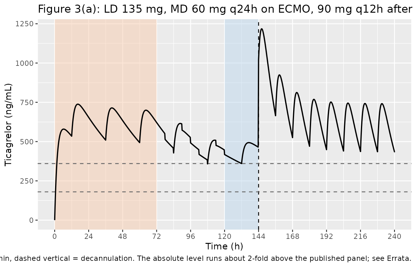
before <- fig3$Cc[which(fig3$time < 144)][sum(fig3$time < 144)]
after  <- fig3$Cc[fig3$time == 144][1]

# Decannulation is a step change in Vd/F only (345.5 L -> 157 L), so the
# concentration jumps by exactly that ratio while the amount is continuous.
jump_expected <- vd_on(1) / vc_off
stopifnot(abs((after / before) / jump_expected - 1) < 0.02)

ss_post <- fig3 |> dplyr::filter(time >= 216, time <= 240)
ss_on   <- fig3 |> dplyr::filter(time >= 48,  time <= 72)

shape <- tibble::tribble(
  ~phase,                                  ~trough_ng,             ~peak_ng,              ~mass_balance_cavg_ng,
  "ON-ECMO 48-72 h (60 mg q24h)",          min(ss_on$Cc)   * 1000, max(ss_on$Cc)   * 1000, 1000 * 60 / (24 * cl_off * e_cl),
  "post-weaning 216-240 h (90 mg q12h)",   min(ss_post$Cc) * 1000, max(ss_post$Cc) * 1000, 1000 * 90 / (12 * cl_off)
)

shape |>
  dplyr::rename(
    "Phase"                       = phase,
    "Trough (ng/mL)"              = trough_ng,
    "Peak (ng/mL)"                = peak_ng,
    "Dose/(tau x CL/F) (ng/mL)"   = mass_balance_cavg_ng
  ) |>
  knitr::kable(digits = 0,
caption = "Simulated Figure 3(a) phases against the mass-balance average.")| Phase | Trough (ng/mL) | Peak (ng/mL) | Dose/(tau x CL/F) (ng/mL) |
|---|---|---|---|
| ON-ECMO 48-72 h (60 mg q24h) | 493 | 700 | 585 |
| post-weaning 216-240 h (90 mg q12h) | 435 | 742 | 615 |
Assumptions and deviations
Encoding decisions
-
Vd/F covariate form – control stream over main
text. The NONMEM control file (Appendix S2
$PK) writesV = THETA(3)*EXP(ETA(2))*THETA(10)**ECMO*(THETA(11)**(LPM/3))**ECMO, so the circuit-flow power term is itself raised to the ECMO indicator and applies only while the patient is cannulated. The main text prints the flow term ungated,Vd/F = 157 * 0.518^(flow/3) * 2.74^ECMO. The control-stream form is encoded because it is the code that was actually run, and because it is robust to howeverQ_ECMOis carried on OFF-ECMO records. The two forms are algebraically identical whenever the delivered circuit flow is zero off ECMO, which is the physically correct coding and the one this model expects; they agree on every ON-ECMO value the paper reports. -
The paper’s “81.3 L OFF-ECMO” is a matched-flow
counterfactual. It equals
222.8 / 2.74, i.e. the main-text equation evaluated at a hypothetical 3 L/min circuit flow in a patient who is not on ECMO. A genuinely decannulated patient has zero circuit flow andVd/F = 157 Lunder either form. The structural verification table reproduces 81.3 explicitly so the paper’s sentence can be audited, but the number should be read as “the ECMO volume effect is 2.74-fold at matched flow”, not as a decannulated volume. -
Concentration units are mg/L, not ng/mL. Appendix
S1 sets
S2 = Vd/FandS3 = VM/Fwith no unit-conversion factor, so with doses in mg and volumes in L the modelled concentration is mg/L. This matters because it fixes the scale of the two additive residual SDs. Three independent checks agree: (i) 0.5218 and 0.06325 mg/L are about 30% and 33% of the corresponding typical steady-state concentrations, a plausible residual magnitude, whereas on a ng/mL reading they would be about 0.03% and arithmetically incompatible with the reported OFV of -1142.42; (ii) their ratio, 8.25, tracks the parent/metabolite concentration ratio of about 9; (iii) the simulated single-180-mg-dose Cmax of about 790 ng/mL parent and 190 ng/mL TAM matches published ticagrelor values. Everything compared against the paper in this vignette is converted with* 1000. -
fmandKaarefixed(). Table 2 prints both with aFIXflag, no RSE and no bootstrap interval. Appendix S3 shows why this is load-bearing for the metabolite: the parent estimates are completely invariant tofm(CL/F 12.2 and Vd/F 157 at everyfmfrom 0.1 to 0.9, identical OFV of -1142.42), whileCLM/FandVM/Fscale in direct proportion to it with an essentially unchangedCLM/VMratio.fmis therefore not identified by these data at all – it was imported from published non-ECMO models – and the absolute values ofCLM/FandVM/Fare conditional on that import, even though the metabolite’s shape and half-life are not. -
Residual error is additive on the linear scale and
fixed. Methods states additive, proportional and combined
models were compared, the proportional component was negligible, and
“residual error parameters were fixed to the preliminary estimates, with
residual variance fixed at 0.1”. The additive SD is therefore
W * sqrt(0.1)per Table 2 footnote c. Note that 0.5218 mg/L is a large additive error relative to the observed concentrations, which is consistent with the positive CWRES skew the paper reports. - No inter-eta covariances. Table 2 reports three diagonal omega-squared terms and no off-diagonals, so the etas are encoded independently.
-
No bioavailability term. All clearances and volumes
are apparent (
/F), so the whole dose entersdepotandFis absorbed intoCL/FandVd/F.
Known deviation: Figure 3 levels are about 2-fold below the published parameters
Simulating the paper’s own 6-day scenario from its own Table 2 parameters puts the typical profile roughly twice as high as the black line in Figure 3, and the 10th-90th percentile band roughly twice as high as the published shaded band. The discrepancy is uniform across both the ON-ECMO segment and the post-weaning segment.
This is a paper-internal inconsistency, not a transcription problem, and it is recorded rather than tuned:
- The packaged model reproduces every printed parameter and every printed derived quantity exactly (structural verification table above, all rows within 0.1%).
- The model satisfies mass balance exactly:
CL/F * AUCinf = Doseto within 0.5% for both analytes in every covariate scenario, and the post-weaning phase of the Figure 3 scenario has a time-average within 5% ofDose / (tau * CL/F). There is no room in the structure for a 2-fold error – the average concentration at steady state is fixed by dose and clearance alone. - The gap is not explained by summarising the cohort
as a population median instead of a typical-value profile. That
distinction is real for this model
(
E[exp(eta_CL - eta_V)] = exp((0.441 + 0.661)/2) = 1.735inflates the effective elimination rate across subjects) but accounts for only about a fifth of the gap: the 200-subject median runs about 490 ng/mL on ECMO against a typical-value 609 ng/mL, where Figure 3(a) shows about 310 ng/mL. - Two further internal checks point the same way. Figure 3 panels (a) and (b) share the identical post-weaning regimen (90 mg q12h) yet do not converge over the 96 h after decannulation, even though the off-ECMO half-life implied by Table 2 is only 8.9 h – more than ten half-lives.
Consequence for the paper’s dosing recommendation. With the published parameters, the recommended on-ECMO regimen (135 mg loading, 60 mg once daily) gives a steady-state trough of roughly 450-500 ng/mL, above the paper’s own 360 ng/mL upper bound, rather than inside the 180-360 ng/mL window as Figure 3 indicates. The paper’s qualitative conclusion is unaffected and is strongly supported by this model: standard 90 mg twice-daily dosing on VA-ECMO gives a simulated median trough far above the target window (see the cohort table above), so a substantial dose reduction is clearly warranted. It is the specific numeric regimen that cannot be re-derived from Table 2 by mass balance. Users who need the dose recommendation itself should treat Figure 3 as the authority and this model as the authority for the parameters; the two are not mutually consistent.
Simulation assumptions
- Original observed concentrations are not public. All figures use virtual cohorts.
- Covariate values in the virtual cohorts are set directly (ECMO status and circuit flow) rather than sampled; the paper reports no distribution for circuit flow – Table 1 does not tabulate it – so the 3.4 L/min and 1 L/min values used here are taken from the paper’s own Monte Carlo scenario definitions in Methods, “Monte Carlo simulations”.
- The covariates screened and rejected by the paper (height, weight, time to start ECMO, ECMO duration, pump speed, BUN, creatinine, uric acid, total protein, albumin, total bilirubin, sex, smoking, CRRT) are not in the model, so no demographic covariates are sampled.
- Cohort assertions are stated on medians and robust quantiles, never on cohort extremes, because rxode2’s RNG stream is partitioned per solver thread and a CI runner draws a different cohort than a workstation.
- All parameter values come from the paper’s text, Table 2, and Appendices S1-S3. No value was digitised from a figure, obtained by correspondence, or carried from another model.