Amlodipine and systolic blood pressure (Mukherjee 2018)
Source:vignettes/articles/Mukherjee_2018_amlodipine.Rmd
Mukherjee_2018_amlodipine.RmdModel and source
- Citation: Mukherjee D, Zha J, Menon RM, Shebley M. (2018). Guiding dose adjustment of amlodipine after co-administration with ritonavir containing regimens using a physiologically-based pharmacokinetic/pharmacodynamic model. J Pharmacokinet Pharmacodyn 45(3):443-456. doi:10.1007/s10928-018-9574-0.
- Article (open access): https://doi.org/10.1007/s10928-018-9574-0
- Supplementary information (Figures S1-S8, Tables S1-S2): https://www.ncbi.nlm.nih.gov/pmc/articles/PMC5953987/
mod <- rxode2::rxode2(readModelDb("Mukherjee_2018_amlodipine"))
WTREF <- 82.2

# The model declares two endpoints (Cc and SBP), so rxode2 needs every
# observation row to identify one of them. Naming a real ODE state in `cmt`
# together with `dvid = 1L` does that and still returns both observables as
# columns; naming the observable itself in `cmt` would renumber the
# compartment slots and is the wrong fix.
prep_events <- function(ev, wt = WTREF, rtv = 0) {
  as.data.frame(ev) |>
    dplyr::mutate(
      cmt = ifelse(evid == 0, "central", as.character(cmt)),
      dvid = 1L,
      id = 1L,
      WT = wt,
      CONMED_RTV = rtv
    )
}
What this model is, and what it is not
Mukherjee 2018 built a minimal PBPK model with a single adjusting compartment (SAC) for amlodipine in Simcyp V15R1, linked it to a systolic-blood-pressure (SBP) pharmacodynamic model implemented as a Lua “custom PD” module, and used the pair to advise on amlodipine dose adjustment around ritonavir (RTV)-containing regimens.
Simcyp’s whole-body mass-balance equations are proprietary and are
not printed. What is printed, in Table 1, is the
complete amlodipine compound layer: ka, the absorption lag,
Vd, V_SAC, Q_SAC, and the
clearance terms. In the Simcyp minimal-PBPK layout the SAC is an
ordinary peripheral compartment with inter-compartmental clearance
Q_SAC, so the disposition reduces exactly to a
two-compartment oral model. That reduction is what this model file
contains – no parameter is fitted, and none is imported from a Simcyp
population file.
The PD layer needs no reduction at all: the authors deposited the Lua source code as supplementary Figure S2, so the equation that generated every published SBP figure is available verbatim.
Three things the model deliberately does not do, all expanded in Assumptions and deviations:
- It does not carry the mechanism of the RTV interaction, only its magnitude.
- It therefore does not reproduce the time course of onset and washout of the interaction (the paper’s Figure 3 and its scenario-2/3 simulations).
- It carries no inter-individual variability and no PK residual error, because the source reports none.
Population
Two-compartment oral pharmacokinetic reduction of the Simcyp minimal-PBPK-with-single-adjusting-compartment (SAC) model for amlodipine, linked to the paper’s own systolic-blood-pressure (SBP) pharmacodynamic model (Mukherjee 2018). The PBPK model was built in Simcyp V15R1 and its whole-body mass-balance equations are not published, but the amlodipine compound layer is reported in full and is sufficient to rebuild the disposition as an ordinary compartmental model: first-order absorption into a depot with a lag time, distribution between a systemic compartment and the SAC (encoded as the canonical peripheral1 with the reported Q_SAC as q), and first-order elimination. Volumes are the reported per-kilogram values (systemic = Vss - V_SAC, peripheral1 = V_SAC) so they scale linearly with body weight. The reduction reproduces the paper’s own predicted single-dose oral Cmax, Tmax, AUC-infinity and terminal half-life and the intravenous AUC-infinity to within 2.6 percent at the back-solved Simcyp population-representative weight of 82.2 kg. The PD layer is transcribed from the Lua script the authors deposited as supplementary Figure S2, which is the code that generated the published figures: SBP is a cosine baseline plus a linear concentration effect that is delayed by an effect-compartment build-up factor 1 - exp(-keo * time-after-first-dose). Note that the main-text Equations 1 and 3 print this factor as exp(-keo * t), which would abolish the drug effect within days and contradicts the sustained day-43 effect the paper shows in Figure 4; the deposited code is taken as authoritative. Ritonavir co-administration enters as the empirical binary covariate CONMED_RTV acting on relative bioavailability and on clearance, calibrated to the paper’s own predicted Cmax and AUC ratios for ritonavir 100 mg once daily (Table 4, Menon row). The mechanistic time-dependent CYP3A4 inhibition and induction that produced those ratios lives in the separate Simcyp ritonavir compound model of Shebley 2017 and is NOT reproducible here, so the time course of onset and washout of the interaction (the paper’s Figure 3) is not captured; see the vignette for the full list of deviations. This is a typical-value simulation model: the source reports no inter-individual variance components and no pharmacokinetic residual error, so there are no etas and propSd is fixed at zero.
The PK layer was optimised against the 12 healthy volunteers of
Faulkner 1986 (intravenous and oral single doses) and the 18 healthy
HIV-seronegative adults of Glesby 2005 (indinavir + RTV interaction),
then verified against four further studies (Table 2 of the paper). The
PD layer was fitted to the mean SBP of the 12
hypertensive patients of Donnelly 1993, aged 25-64 years, given
amlodipine 5 mg once daily for six weeks; only means were published, so
no between-subject variability could be estimated even though the paper
states it was high for m and keo.
Every simulation in the paper uses the Simcyp “population representative” virtual subject – one typical individual, not a sampled population – which is why the model below has no etas.
Source trace
| Model element | Value | Source location |
|---|---|---|
lka |
0.75 1/h | Table 1, Optimized parameters, absorption rate constant |
ltlag |
3.2 h | Table 1, Optimized parameters, absorption lag time |
lfdepot |
0.666 | Table 4, Faulkner (oral) row, predicted F = 66.6% |
lcl |
33.9 L/h | Table 1, Initial estimates, IV clearance (Faulkner 1986) |
lvc |
854.88 L | Table 1: (Vd 21.4 - V_SAC 11) L/kg x 82.2 kg |
lvp |
904.2 L | Table 1, Optimized parameters: V_SAC 11 L/kg x 82.2 kg |
lq |
90 L/h | Table 1, Optimized parameters: Q_SAC = 90 L/h |
e_wt_vc_vp |
1 | Structural: Table 1 reports both volumes in L/kg |
| 82.2 kg reference weight | 82.2 kg | Not printed. Back-solved from the predicted terminal half-life of 39.9 h (Table 4) |
e_conmed_rtv_fdepot |
1.3783 | Back-solved from Table 4, Menon row (Cmax ratio 1.42, AUC ratio 2.28) |
e_conmed_rtv_cl |
0.6045 | Back-solved from the same pair |
le0 |
148.84 mmHg | Figure S2 Lua script Po; Table 3 prints 148.8 |
lamp |
8.245 mmHg | Figure S2 Lua script A; Table 3 prints 8.25 |
lfcirc |
1.76 1/day | Table 3, circadian frequency |
lke0 |
0.049 1/h | Table 3 and Figure S2 Lua script keo
|
slope_drug |
-3.145 mmHg per ng/mL | Table 3, m
|
addSd_SBP |
5.04 mmHg | Table 3, drug-effect block, residual-error column (RMSE, footnote c) |
propSd |
0 (fixed) | Not reported; deterministic platform simulation |
| SBP equation | Equation 3 | Main text Eq. 3, implemented as Figure S2 |
| Disposition ODEs | two-compartment | Reduction of the Figure 1b minimal-PBPK + SAC layout |
Two arithmetic cross-checks of the PD transcription
Table 3 and the Lua script state the same two parameters in different units. Both conversions close exactly, which is strong evidence that the transcription is right.
mw_amlodipine <- 408.88 # g/mol, Table 1
m_table3 <- -3.145      # mmHg per ng/mL, Table 3
m_lua <- -1285.93       # mmHg per uM, Figure S2 Lua script
f_table3 <- 1.76        # cycles/day, Table 3
om_lua <- 0.463         # 1/h, Figure S2 Lua script

stopifnot(
  abs(m_table3 * mw_amlodipine / m_lua - 1) < 1e-4,
  abs(2 * pi * f_table3 / 24 / om_lua - 1) < 5e-3
)
cat(sprintf("m: %.3f mmHg/(ng/mL) x %.2f g/mol = %.2f mmHg/uM (Lua %.2f)\n",
            m_table3, mw_amlodipine, m_table3 * mw_amlodipine, m_lua))
#> m: -3.145 mmHg/(ng/mL) x 408.88 g/mol = -1285.93 mmHg/uM (Lua -1285.93)
cat(sprintf("f: 2*pi*%.2f/24 = %.4f 1/h (Lua %.3f)\n",
            f_table3, 2 * pi * f_table3 / 24, om_lua))
#> f: 2*pi*1.76/24 = 0.4608 1/h (Lua 0.463)
Single-dose pharmacokinetics
Four typical-subject arms: the two Faulkner 1986 10 mg arms the model was optimised against, and the two 5 mg arms of the Menon 2015 RTV interaction study.
grid_sd <- c(seq(0, 24, by = 0.05), seq(24.5, 720, by = 0.5))

make_arm <- function(arm, amt, route, rtv) {
  ev <- if (route == "iv") {
    rxode2::et(amt = amt, cmt = "central", dur = 1 / 6)
  } else {
    rxode2::et(amt = amt, cmt = "depot")
  }
  ev <- rxode2::et(ev, grid_sd)
  prep_events(ev, rtv = rtv) |> dplyr::mutate(arm = arm)
}

events_sd <- dplyr::bind_rows(
  make_arm("IV 10 mg (10 min)", 10, "iv", 0),
  make_arm("Oral 10 mg", 10, "po", 0),
  make_arm("Oral 5 mg", 5, "po", 0),
  make_arm("Oral 5 mg + RTV", 5, "po", 1)
) |>
  dplyr::mutate(id = as.integer(factor(arm)))

sim_sd <- rxode2::rxSolve(mod, events_sd, returnType = "data.frame") |>
  dplyr::left_join(dplyr::distinct(events_sd, id, arm), by = "id")
#> Warning: multi-subject simulation without without 'omega'

ggplot(dplyr::filter(sim_sd, time <= 120),
       aes(time, Cc, colour = arm)) +
  geom_line() +
  scale_y_log10() +
  labs(x = "Time (h)", y = "Amlodipine (ng/mL)", colour = NULL,
       title = "Replicates Figure 1a-b of Mukherjee 2018 (model predictions)")
#> Warning in scale_y_log10(): log-10 transformation introduced infinite values.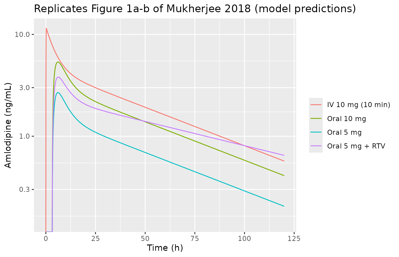
PKNCA validation
conc_sd <- sim_sd |>
  dplyr::filter(!is.na(Cc)) |>
  dplyr::select(id, time, Cc, arm)

# Guarantee a time-zero record per arm so PKNCA does not extrapolate the AUC
# start before the first measurement.
conc_sd <- dplyr::bind_rows(
  conc_sd,
  conc_sd |> dplyr::distinct(id, arm) |> dplyr::mutate(time = 0, Cc = 0)
) |>
  dplyr::distinct(id, arm, time, .keep_all = TRUE) |>
  dplyr::arrange(id, arm, time)

dose_sd <- events_sd |>
  dplyr::filter(evid != 0) |>
  dplyr::select(id, time, amt, arm)

nca_sd <- PKNCA::pk.nca(PKNCA::PKNCAdata(
  PKNCA::PKNCAconc(conc_sd, Cc ~ time | arm + id,
                   concu = "ng/mL", timeu = "h"),
  PKNCA::PKNCAdose(dose_sd, amt ~ time | arm + id, doseu = "mg"),
  intervals = data.frame(
    start      = 0,
    end        = Inf,
    cmax       = TRUE,
    tmax       = TRUE,
    aucinf.obs = TRUE,
    half.life  = TRUE
  )
))

nca_tbl <- as.data.frame(nca_sd) |>
  dplyr::filter(PPTESTCD %in% c("cmax", "tmax", "aucinf.obs", "half.life")) |>
  dplyr::mutate(PPORRES = signif(PPORRES, 4))

knitr::kable(
  nca_tbl |> dplyr::select(arm, PPTESTCD, PPORRES),
  caption = "PKNCA results for the four simulated single-dose arms."
)| arm | PPTESTCD | PPORRES |
|---|---|---|
| IV 10 mg (10 min) | cmax | 11.500 |
| IV 10 mg (10 min) | tmax | 0.200 |
| IV 10 mg (10 min) | half.life | 39.680 |
| IV 10 mg (10 min) | aucinf.obs | 295.000 |
| Oral 10 mg | cmax | 5.362 |
| Oral 10 mg | tmax | 6.100 |
| Oral 10 mg | half.life | 39.670 |
| Oral 10 mg | aucinf.obs | 196.500 |
| Oral 5 mg | cmax | 2.681 |
| Oral 5 mg | tmax | 6.100 |
| Oral 5 mg | half.life | 39.670 |
| Oral 5 mg | aucinf.obs | 98.230 |
| Oral 5 mg + RTV | cmax | 3.807 |
| Oral 5 mg + RTV | tmax | 6.250 |
| Oral 5 mg + RTV | half.life | 62.950 |
| Oral 5 mg + RTV | aucinf.obs | 224.000 |
Comparison against the paper’s own predicted values
Table 4 of Mukherjee 2018 reports model-predicted PK parameters for the Faulkner 1986 arms. Those are the right comparator: the target is the published model’s output, not the clinical observations, because the object here is to show that the two-compartment reduction reproduces the Simcyp model.
published_sd <- tibble::tribble(
  ~arm,                 ~cmax, ~tmax, ~aucinf.obs, ~half.life,
  "IV 10 mg (10 min)",     NA,    NA,         303,       39.9,
  "Oral 10 mg",          5.45,  6.09,         201,       39.9
)

cmp_sd <- nlmixr2lib::ncaComparisonTable(
  simulated = nca_tbl |> dplyr::filter(arm %in% published_sd$arm),
  reference = published_sd,
  by        = "arm",
  units     = c(cmax = "ng/mL", tmax = "h",
                aucinf.obs = "ng*h/mL", half.life = "h"),
  tolerance_pct = 20
)

knitr::kable(
  cmp_sd,
  caption = paste("Simulated vs. Mukherjee 2018 Table 4 model-predicted",
                  "values. * marks a difference over 20%."),
  align = c("l", "l", "r", "r", "r")
)| NCA parameter | arm | Reference | Simulated | % diff |
|---|---|---|---|---|
| Cmax (ng/mL) | IV 10 mg (10 min) | — | 11.5 | — |
| Cmax (ng/mL) | Oral 10 mg | 5.45 | 5.36 | -1.6% |
| Tmax (h) | IV 10 mg (10 min) | — | 0.2 | — |
| Tmax (h) | Oral 10 mg | 6.09 | 6.1 | +0.2% |
| AUC0-∞ (obs) (ng*h/mL) | IV 10 mg (10 min) | 303 | 295 | -2.6% |
| AUC0-∞ (obs) (ng*h/mL) | Oral 10 mg | 201 | 196 | -2.2% |
| t½ (h) | IV 10 mg (10 min) | 39.9 | 39.7 | -0.6% |
| t½ (h) | Oral 10 mg | 39.9 | 39.7 | -0.6% |
pct <- suppressWarnings(
  as.numeric(gsub("[^0-9.eE+-]", "", as.character(cmp_sd[["% diff"]])))
)
# A tight bound is correct here: every arm is the same deterministic typical
# subject, so there is no cohort draw for a CI to protect against. The residual
# is the reduction's own approximation error, not sampling noise.
stopifnot(any(is.finite(pct)), max(abs(pct), na.rm = TRUE) < 5)
cat(sprintf(paste("All %d comparisons against Mukherjee 2018 Table 4 agree;",
                  "largest discrepancy %.1f%%.\n"),
            sum(is.finite(pct)), max(abs(pct), na.rm = TRUE)))
#> All 6 comparisons against Mukherjee 2018 Table 4 agree; largest discrepancy 2.6%.
The paper additionally reports a predicted oral bioavailability of 66.6%, which is an input here rather than an output, and a predicted IV Cmax it describes as substantially under-predicted relative to observation; neither is a test of the reduction.
The ritonavir interaction is calibrated, not predicted
The two CONMED_RTV coefficients were back-solved so that
the single 5 mg dose reproduces the paper’s Table 4 Menon row. This
block is therefore a consistency check on the encoding, not
independent evidence.
ddi <- nca_tbl |>
  dplyr::filter(arm %in% c("Oral 5 mg", "Oral 5 mg + RTV"),
                PPTESTCD %in% c("cmax", "aucinf.obs")) |>
  dplyr::select(arm, PPTESTCD, PPORRES) |>
  tidyr::pivot_wider(names_from = arm, values_from = PPORRES) |>
  dplyr::mutate(
    ratio = .data[["Oral 5 mg + RTV"]] / .data[["Oral 5 mg"]],
    published = c(1.42, 2.28)[match(PPTESTCD, c("cmax", "aucinf.obs"))]
  )

knitr::kable(
  ddi |> dplyr::rename("NCA parameter" = PPTESTCD,
                       "Simulated ratio" = ratio,
                       "Mukherjee 2018 Table 4" = published),
  digits = 3,
  caption = "Amlodipine exposure ratio with ritonavir 100 mg once daily."
)| NCA parameter | Oral 5 mg | Oral 5 mg + RTV | Simulated ratio | Mukherjee 2018 Table 4 |
|---|---|---|---|---|
| cmax | 2.681 | 3.807 | 1.42 | 1.42 |
| aucinf.obs | 98.230 | 224.000 | 2.28 | 2.28 |
Multiple-dose pharmacokinetics: accumulation
Faulkner 1986 also gave 15 mg once daily for 14 days to 28 healthy subjects. Mukherjee 2018 Results report model-predicted accumulation ratios (day 14 : day 1) of 2.1 for Cmax and 2.9 for AUC24. These are genuine held-out targets – nothing in this reduction was calibrated to them.
ev_md <- rxode2::et(amt = 15, cmt = "depot", ii = 24, addl = 13) |>
  rxode2::et(seq(0, 336, by = 0.05))
events_md <- prep_events(ev_md)

sim_md <- rxode2::rxSolve(mod, events_md, returnType = "data.frame")

day <- function(d) dplyr::filter(sim_md, time >= (d - 1) * 24, time <= d * 24)
trapz <- function(x) sum(diff(x$time) * (head(x$Cc, -1) + tail(x$Cc, -1)) / 2)

acc <- tibble::tibble(
  Metric = c("Cmax", "AUC24"),
  Simulated = c(max(day(14)$Cc) / max(day(1)$Cc), trapz(day(14)) / trapz(day(1))),
  `Mukherjee 2018` = c(2.1, 2.9)
)
knitr::kable(acc, digits = 2,
caption = "Accumulation ratio, day 14 : day 1, 15 mg once daily.")| Metric | Simulated | Mukherjee 2018 |
|---|---|---|
| Cmax | 2.07 | 2.1 |
| AUC24 | 2.76 | 2.9 |
stopifnot(max(abs(acc$Simulated / acc$`Mukherjee 2018` - 1)) < 0.10)

ggplot(sim_md, aes(time / 24, Cc)) +
  geom_line() +
  labs(x = "Time (days)", y = "Amlodipine (ng/mL)",
       title = "Replicates Figure 1c/1f: 15 mg once daily for 14 days")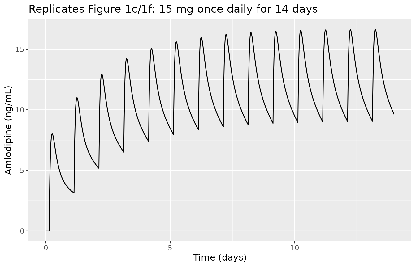
Steady state is reached at about day 7, as the paper reports.
Systolic blood pressure
Baseline rhythm and the effect build-up
With no drug, SBP oscillates about P0 with amplitude
A. Note that the fitted frequency is 1.76 cycles per day,
i.e. a period of about 13.6 h, and that the phase argument is reset to
zero at each midnight boundary – both are properties of the published
equation as the authors implemented it, not choices made here.
ev_pd0 <- rxode2::et(amt = 0, cmt = "depot") |>
  rxode2::et(seq(0, 48, by = 0.1))
sim_pd0 <- rxode2::rxSolve(mod, prep_events(ev_pd0), returnType = "data.frame")

stopifnot(
  abs(max(sim_pd0$SBP) - (148.84 + 8.245)) < 0.05,
  abs(min(sim_pd0$SBP) - (148.84 - 8.245)) < 0.5
)

ggplot(sim_pd0, aes(time, SBP)) +
  geom_line() +
  labs(x = "Time (h)", y = "SBP (mmHg)",
       title = "Drug-free baseline rhythm (Equation 2)")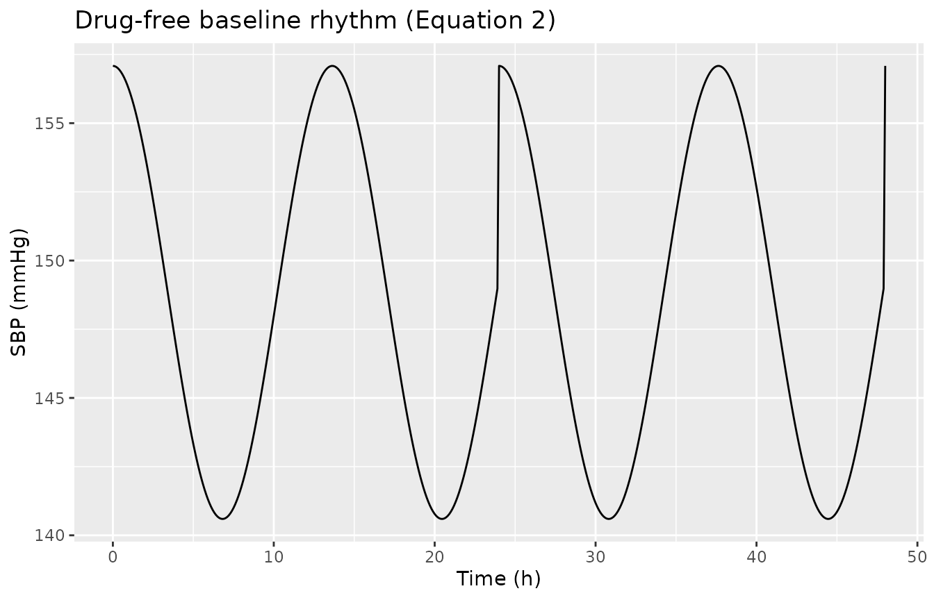
Scenario 1 (Figure 5): dose adjustment during ritonavir
Amlodipine 5 mg once daily for 14 days alone, then ritonavir 100 mg once daily added for 14 days with the amlodipine dose either kept at 5 mg or halved to 2.5 mg.
rtv_on <- function(tt) as.numeric(tt >= 14 * 24 & tt < 28 * 24)

scenario1 <- function(dose_with_rtv, label) {
  ev <- rxode2::et(amt = 5, cmt = "depot", ii = 24, addl = 13) |>
    rxode2::et(amt = dose_with_rtv, cmt = "depot", time = 14 * 24,
               ii = 24, addl = 13) |>
    rxode2::et(seq(0, 28 * 24, by = 0.2))
  prep_events(ev) |>
    dplyr::mutate(CONMED_RTV = rtv_on(time), arm = label)
}

events_s1 <- dplyr::bind_rows(
  scenario1(5, "No dose adjustment (5 mg QD throughout)"),
  scenario1(2.5, "Dose adjusted (2.5 mg QD with RTV)")
) |>
  dplyr::mutate(id = as.integer(factor(arm)))

sim_s1 <- rxode2::rxSolve(mod, events_s1, returnType = "data.frame") |>
  dplyr::left_join(dplyr::distinct(events_s1, id, arm), by = "id")
#> Warning: multi-subject simulation without without 'omega'

ggplot(sim_s1, aes(time / 24, Cc, colour = arm)) +
  geom_line() +
  geom_vline(xintercept = c(14, 28), linetype = 2) +
  labs(x = "Time (days)", y = "Amlodipine (ng/mL)", colour = NULL,
       title = "Replicates Figure 5a of Mukherjee 2018")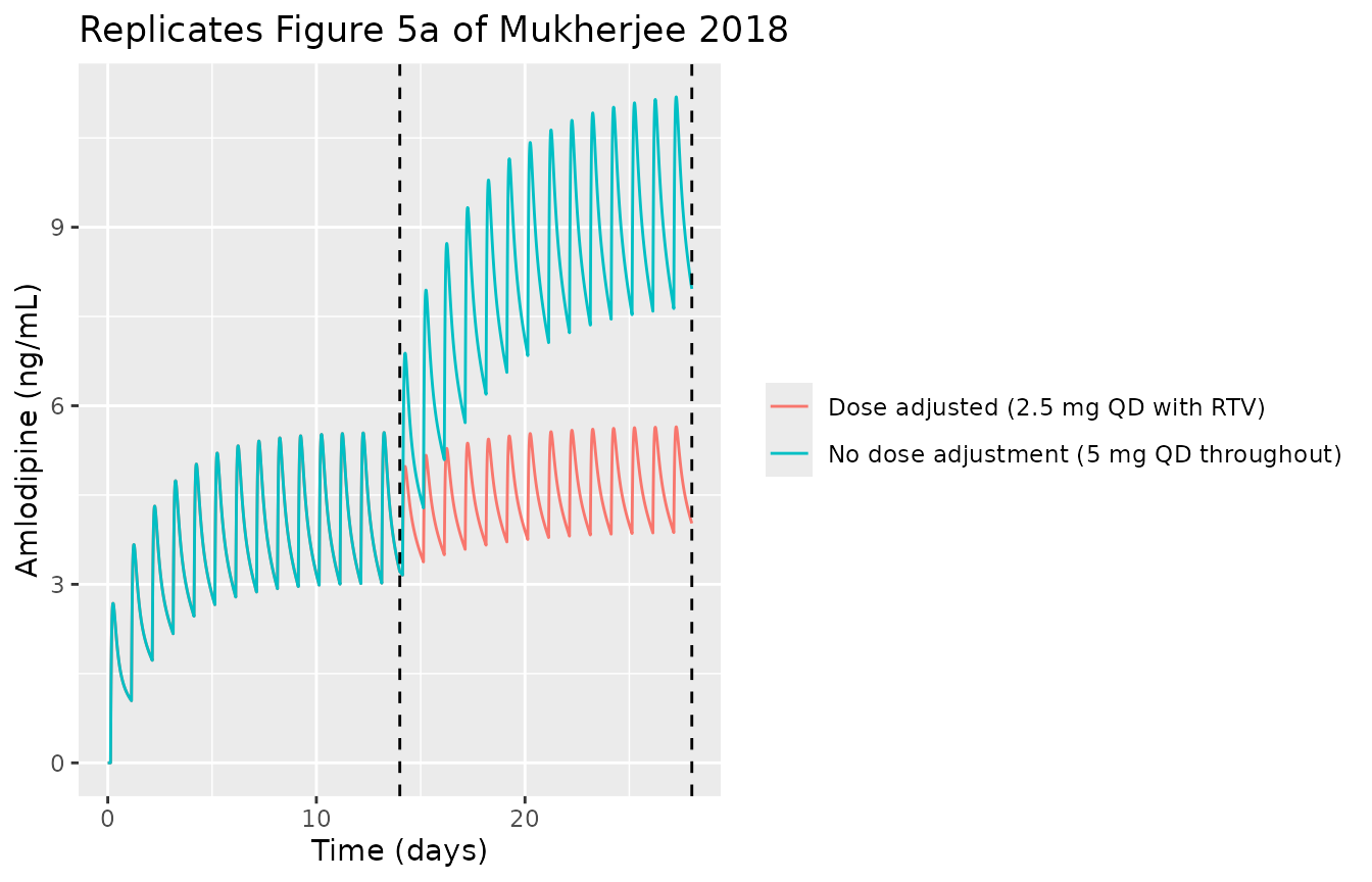
ggplot(sim_s1, aes(time / 24, SBP, colour = arm)) +
  geom_line() +
  geom_hline(yintercept = 110, linetype = 3) +
  geom_vline(xintercept = c(14, 28), linetype = 2) +
  labs(x = "Time (days)", y = "SBP (mmHg)", colour = NULL,
       title = "Replicates Figure 5b of Mukherjee 2018")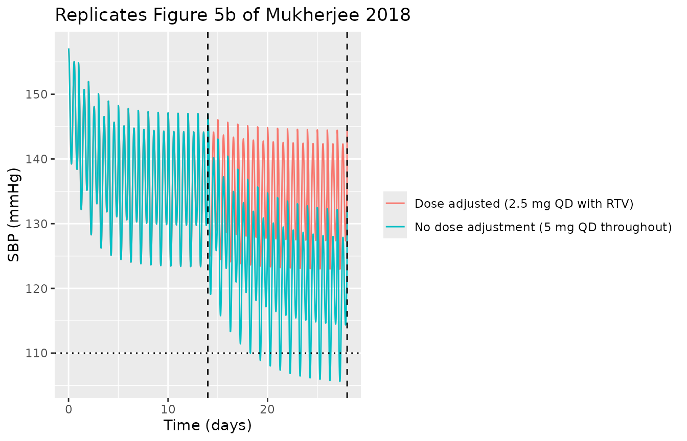
The paper makes three checkable statements about this scenario. All three are held out – the model was calibrated only to the Table 4 exposure ratios.
with_rtv <- dplyr::filter(sim_s1, time >= 24 * 24, time <= 28 * 24)
noadj <- dplyr::filter(with_rtv, arm == "No dose adjustment (5 mg QD throughout)")
adj <- dplyr::filter(with_rtv, arm == "Dose adjusted (2.5 mg QD with RTV)")
before <- dplyr::filter(sim_s1, time >= 10 * 24, time <= 14 * 24,
                        arm == "Dose adjusted (2.5 mg QD with RTV)")

checks <- tibble::tibble(
  Statement = c(
    "Without dose adjustment, SBP drops below 110 mmHg",
    "With dose adjustment, amlodipine exposure is maintained",
    "With dose adjustment, SBP is maintained"
  ),
  `Mukherjee 2018` = c("< 110 mmHg", "same level as before RTV",
                       "similar level to before RTV"),
  Simulated = c(
    sprintf("min %.1f mmHg", min(noadj$SBP)),
    sprintf("mean Cc %.2f vs %.2f ng/mL", mean(adj$Cc), mean(before$Cc)),
    sprintf("mean SBP %.1f vs %.1f mmHg", mean(adj$SBP), mean(before$SBP))
  )
)
knitr::kable(checks, caption = "Held-out qualitative checks for scenario 1.")| Statement | Mukherjee 2018 | Simulated |
|---|---|---|
| Without dose adjustment, SBP drops below 110 mmHg | < 110 mmHg | min 105.6 mmHg |
| With dose adjustment, amlodipine exposure is maintained | same level as before RTV | mean Cc 4.63 vs 4.07 ng/mL |
| With dose adjustment, SBP is maintained | similar level to before RTV | mean SBP 133.6 vs 135.4 mmHg |
The 2.5 mg plateau the paper quotes for scenario 2
Scenario 2 continues 2.5 mg once daily for five days after the last ritonavir dose, and the paper quotes a maximum SBP of 149.9 mmHg reached over those five days. The interaction is still washing out over that window, so 149.9 mmHg must sit below the ritonavir-free 2.5 mg once-daily plateau, which this model can compute.
ev_25 <- rxode2::et(amt = 2.5, cmt = "depot", ii = 24, addl = 59) |>
  rxode2::et(seq(59 * 24, 60 * 24, by = 0.1))
sim_25 <- rxode2::rxSolve(mod, prep_events(ev_25), returnType = "data.frame") |>
  dplyr::filter(time >= 59 * 24)

cat(sprintf(paste("Ritonavir-free 2.5 mg QD plateau: SBP max %.1f mmHg.",
                  "Mukherjee 2018 scenario 2 quotes 149.9 mmHg five days",
                  "after the last RTV dose, i.e. still below it.\n"),
            max(sim_25$SBP)))
#> Ritonavir-free 2.5 mg QD plateau: SBP max 152.0 mmHg. Mukherjee 2018 scenario 2 quotes 149.9 mmHg five days after the last RTV dose, i.e. still below it.
stopifnot(max(sim_25$SBP) > 149.9, max(sim_25$SBP) < 160)
Assumptions and deviations
Reference body weight (82.2 kg) is not printed in the paper. Table 1 gives both distribution volumes per kilogram, so a body weight is needed to turn them into litres, and the paper only says that the Simcyp “population representative” healthy volunteer was used. The weight was obtained by requiring the reduction to return the paper’s own predicted terminal half-life of 39.9 h (Table 4). The four remaining printed predictions were then held out as an audit and are reproduced to within 2.6%. Users simulating a different body weight get linearly scaled volumes and a proportionally scaled terminal half-life, because the paper’s clearances are absolute (L/h) while its volumes are per kilogram.
The liver and portal-vein volumes of the Simcyp layout are not subtracted from the systemic compartment. They are not reported; together they are under 0.3% of the 855 L systemic volume, well inside the residual of the audit above.
The ritonavir interaction is empirical.
CONMED_RTV is a binary steady-state switch whose two
coefficients were back-solved from the paper’s own predicted Cmax and
AUC ratios for ritonavir 100 mg once daily. The mechanism that produced
those ratios – reversible plus mechanism-based CYP3A4 inhibition
together with CYP3A4 induction – lives in the separate Simcyp ritonavir
compound model of Shebley 2017, which is a platform artefact and is not
obtainable as published equations.
Two consequences follow, and they are the main limitation of this file:
- The time course of the interaction, which is the
paper’s headline result (Figure 3: the DDI ratio falls to 1.2 by day 34,
five days after the last RTV dose), cannot be reproduced. Switching
CONMED_RTVfrom 1 to 0 is instantaneous. - Scenarios 2 and 3 of the paper – which compare resuming the full amlodipine dose immediately versus five days after the last RTV dose – are therefore not replicated. Their quoted SBP extremes (149.9 and 119.9 mmHg for the 5 mg scenario, 98.5 mmHg for the 10 mg scenario) all sit between this model’s RTV-on and RTV-off plateaus, which is the most that can be checked; the 2.5 mg bound is the one shown above.
The paper’s other interaction arm is not encoded. Table 4 also reports predicted ratios for indinavir 800 mg twice daily plus ritonavir 100 mg twice daily (Cmax ratio 1.74, AUC24 ratio 1.89). That is a different perpetrator combination at a different ritonavir dose and schedule, so folding it into the same binary column would be wrong. A future model that needs it should carry a second covariate.
The main text and the deposited code disagree, and the code
was followed. Equations 1 and 3 print the drug term as
m * C * exp(-keo * t), which decays to nothing within days;
the Lua script of Figure S2 – the code that generated the published
figures – has m * xin * (1 - exp(-keo * t)), an
effect-compartment build-up factor. Only the latter is consistent with
Figure 4, where the day-43 SBP depression is larger than the day-1
depression, and with the paper’s own description of keo as
accounting for “the delay between amlodipine plasma exposure and the
lowering of blood pressure”. The supplement’s form is used here.
The circadian term is periodic with a 13.6 h period, not 24
h, and resets at midnight. f = 1.76 cycles/day is
a fitted parameter (Table 3), and the Lua script evaluates
cos(om * (t - 24 * floor(t / 24))), so the argument jumps
back to zero at each 24 h boundary. This is encoded exactly as
published; it is unusual for a circadian model and is worth knowing
before reusing the baseline term elsewhere.
No inter-individual variability and no PK residual
error. The source is a deterministic simulation of one
population representative, and reports neither. propSd is
fixed at zero. The SBP additive residual SD of 5.04 mmHg is the
root-mean-squared error of the PD fit reported in Table 3 (footnote c),
which is a goodness-of-fit statistic rather than an estimated
$SIGMA; it is carried because it is the only dispersion the
paper reports for the endpoint.
The clearance pathway split is not encoded. Table 1
apportions clearance across CYP3A4 (intrinsic 170 L/h), CYP3A5 (43.5
L/h), biliary (12 L/h), non-specific systemic (16 L/h) and renal (1.8
L/h) routes. In a compartmental reduction with a fixed total clearance
the split is kinetically inert – it cannot change Cc – and
the values are recorded in the model’s population metadata
instead. It also cannot be turned into the interaction term: the printed
apportionment, run through the well-stirred liver model, caps the
attainable AUC ratio for complete CYP3A inhibition below the 2.28 the
paper predicts, which is one more sign that the interaction depends on
platform internals that are not available.
Enterohepatic recirculation is not carried. Table S1 lists biliary clearance as an assumption motivated by reported enterohepatic recycling of amlodipine, and records its implication as “no significant effect”. The reduction folds it into total clearance.