Warfarin (Rodriguez-Fernandez 2024)
Source:vignettes/articles/RodriguezFernandez_2024_warfarin.Rmd
RodriguezFernandez_2024_warfarin.RmdModel and source
- Citation: Rodriguez-Fernandez K, Reynaldo-Fernandez G, Reyes-Gonzalez S, de las Barreras C, Rodriguez-Vera L, Vlaar C, Monbaliu J-CM, Stelzer T, Duconge J, Mangas-Sanjuan V. New insights into the role of VKORC1 polymorphisms for optimal warfarin dose selection in Caribbean Hispanic patients through an external validation of a population PK/PD model. Biomed Pharmacother. 2024;170:115977. doi:10.1016/j.biopha.2023.115977. PMID: 38056237. PMCID: PMC10853672. PD parameters from Table 2; Imax, INRmax, transit-chain length and the fixed MTT values from the Results (‘Base population PK/PD model’ and ‘Final population PK/PD model’). The PK layer is fixed (no IIV) from the upstream publication Reyes-Gonzalez S, de las Barreras C, Reynaldo G, Rodriguez-Vera L, Vlaar C, Lopez Mejias V, Monbaliu J-CM, Stelzer T, Mangas V, Duconge J. Genotype-driven pharmacokinetic simulations of warfarin levels in Puerto Ricans. Drug Metab Pers Ther. 2020;35(4). doi:10.1515/dmpt-2020-0135. PMID: 34704696. PMCID: PMC7892629 (Methods: ka, F, Vd/kg and the six CYP2C9-genotype elimination rate constants). The transit-chain / INR structural form follows Hamberg 2007 and Hamberg 2010; see modellib(‘Hamberg_2007_warfarin_s’).
- Description: Warfarin population PK/PD model for INR in Caribbean Hispanic (Puerto Rican) patients: a one-compartment first-order-oral PK layer fixed from Reyes-Gonzalez 2020 (CYP2C9-genotype-specific elimination rate constant, weight-proportional volume) driving an inhibitory sigmoid-Imax effect on the zero-order synthesis rate of two parallel three-compartment transit chains, combined into INR. VKORC1 -1639G>A is a predictor of both the baseline INR and the warfarin IC50, the latter modelled as a sum of per-allele contributions. Caribbean Hispanic IC50 values are 3-5x higher than previously published European estimates.
- Article: https://doi.org/10.1016/j.biopha.2023.115977 (PMC10853672)
- Upstream PK publication: https://doi.org/10.1515/dmpt-2020-0135 (PMC7892629)
This is an external-validation paper. The authors did not measure warfarin concentrations; they fixed a published one-compartment genotype-driven PK model (Reyes-Gonzalez 2020, same Puerto Rican patient registry) and re-estimated a Hamberg-style INR pharmacodynamic model on 1033 INR observations from 138 Caribbean Hispanic patients. Consequently the PK layer carries no inter-individual variability: every subject sharing a CYP2C9 genotype and a body weight has an identical concentration-time profile.
The headline finding is that the warfarin IC50 in this cohort (9.22-11.76 mg/L depending on VKORC1 haplotype) is three to five times higher than the 1.56-3.11 mg/L reported for European cohorts, i.e. Caribbean Hispanic patients appear substantially more warfarin-resistant.
Population
The analysis dataset comprised 1033 INR observations from 138 patients followed at the Veterans Affairs Caribbean Healthcare System anticoagulation clinic in San Juan, Puerto Rico, over more than 2000 days. Patients were elderly and predominantly male (median age 68 years, range 31-90; median body weight 83 kg, range 51-159 kg); the paper states “mostly males” but reports no sex breakdown. Self-reported race was White Hispanic 24%, Black Hispanic 19%, Admixed 27%, and other or not reported 30%. Total weekly warfarin doses ranged from 7 to 82 mg on a 24- or 48-hour dosing interval (Rodriguez-Fernandez 2024, Table 1).
Eight CYP2C9 diplotypes were observed (*1/*1 71%, *1/*2 15%, *1/*3 5.1%, *1/*5 0.72%, *1/*8 1.44%, *2/*2 1.44%, *2/*3 4.34%, *2/*5 0.72%) and three VKORC1 -1639G>A haplotypes (G/A 45%, G/G 41.3%, A/A 13.7%). The presence of *5 and *8 carriers is a feature of this admixed cohort that the European Hamberg warfarin models do not cover.
The same information is available programmatically via
readModelDb("RodriguezFernandez_2024_warfarin")()$population.
Source trace
The per-parameter origin is recorded as an in-file comment next to
each ini() entry in
inst/modeldb/specificDrugs/RodriguezFernandez_2024_warfarin.R.
The table below collects them in one place. Note that the PK
layer is not from this paper: Rodriguez-Fernandez 2024 fixes it
wholesale from Reyes-Gonzalez 2020 and reports no PK parameter values of
its own.
| Equation / parameter | Value | Source location |
|---|---|---|
lka (ka) |
1.19 1/h | Reyes-Gonzalez 2020, Methods / Study Design (fixed from the literature) |
lvc (Vd per kg) |
0.14 L/kg | Reyes-Gonzalez 2020, Methods / Study Design (population average from the literature; F assumed 100%) |
lkel_11 |
0.0189 1/h | Reyes-Gonzalez 2020, Methods (CYP2C9 *1/*1) |
lkel_12 |
0.0158 1/h | Reyes-Gonzalez 2020, Methods (*1/*2) |
lkel_1n |
0.0132 1/h | Reyes-Gonzalez 2020, Methods (*1/*n, n in {*3,*5,*6,*8}) |
lkel_22 |
0.0130 1/h | Reyes-Gonzalez 2020, Methods (*2/*2) |
lkel_2n |
0.0090 1/h | Reyes-Gonzalez 2020, Methods (*2/*n) |
lkel_nn |
0.0075 1/h | Reyes-Gonzalez 2020, Methods (*n/*n) |
lmtt1 |
27.2 h (1.13 d) | Table 2 (FIX); hour equivalent from Results, “Base population PK/PD model” |
lmtt2 |
110.9 h (4.62 d) | Table 2 (FIX); hour equivalent from Results, “Base population PK/PD model” |
lrbase_ga |
1.78 | Table 2, Baseline G/A |
lrbase_gg |
1.84 | Table 2, Baseline G/G |
lrbase_aa |
2.18 | Table 2, Baseline A/A |
lec50_g |
5.88 mg/L per G allele | Table 2, IC50 G |
lec50_a |
4.61 mg/L per A allele | Table 2, IC50 A |
lhill (gamma) |
1.47 | Table 2, gamma |
limax |
1 (100%) | Results, “Base population PK/PD model” (“complete (100%) inhibition … (Imax)”) |
linrmax |
20 | Results, “Base population PK/PD model” (“the maximum INR was set to 20”) |
etalrbase |
CV 23% | Table 2, IIV Baseline |
etalec50 |
CV 34% | Table 2, IIV IC50 |
propSd |
0.27 | Table 2, RUV Proportional |
| One-compartment first-order oral PK | n/a | Reyes-Gonzalez 2020, Methods (single- and multiple-dose closed-form equations) |
| Two three-compartment transit chains | n/a | Results, “Base population PK/PD model” (“two transit compartment chains with three compartments each”) |
| Inhibitory sigmoid Imax on zero-order synthesis | n/a | Results, “Base population PK/PD model” |
| IC50 as a sum of per-allele contributions | n/a | Results, “Final population PK/PD model” (“modelled by accounting for the effects of individual alleles (G and A)”) |
INR observation rbase + INRmax * (1 - A3 * B3)
|
n/a | Hamberg 2007 / 2010 form; no INR-response exponent is reported in Table 2 – see “Assumptions and deviations” |
Virtual cohort
Original patient-level data are not publicly available. The cohorts below are virtual populations built at the cohort median body weight (83 kg) so that the genotype contrast is not confounded by weight.
# set.seed() seeds R's RNG. It does NOT seed rxode2's simulation RNG, and
# rxode2's streams are partitioned PER SOLVER THREAD, so this cohort is
# reproducible on this machine and different on a machine with a different
# thread count. Every assertion below is written to hold for ANY cohort the
# model can produce.
set.seed(20240201)

# The eight CYP2C9 diplotypes observed in the cohort, as per-allele counts.
cyp_geno <- tibble::tribble(
  ~cyp,     ~S1, ~S2, ~S3, ~S5, ~S6, ~S8,
  "*1/*1",    2,   0,   0,   0,   0,   0,
  "*1/*2",    1,   1,   0,   0,   0,   0,
  "*1/*3",    1,   0,   1,   0,   0,   0,
  "*1/*5",    1,   0,   0,   1,   0,   0,
  "*1/*8",    1,   0,   0,   0,   0,   1,
  "*2/*2",    0,   2,   0,   0,   0,   0,
  "*2/*3",    0,   1,   1,   0,   0,   0,
  "*2/*5",    0,   1,   0,   1,   0,   0
)

vk_geno <- tibble::tibble(
  vkorc1 = c("G/G", "G/A", "A/A"),
  VKORC1_1639G_COUNT = c(2, 1, 0)
)

# Every CYP2C9 count column must be present on every row, and the six counts
# must sum to 2 for each subject -- the model's diplotype indicators are only
# mutually exclusive under that invariant.
stopifnot(all(rowSums(cyp_geno[, c("S1", "S2", "S3", "S5", "S6", "S8")]) == 2))

WT_MEDIAN <- 83  # Rodriguez-Fernandez 2024 Table 1, median body weight (kg)

#' Attach the model's covariate columns to a subject-level frame.
add_covariates <- function(x) {
  dplyr::mutate(
    x,
    WT = WT_MEDIAN,
    CYP2C9_S1_COUNT = S1, CYP2C9_S2_COUNT = S2, CYP2C9_S3_COUNT = S3,
    CYP2C9_S5_COUNT = S5, CYP2C9_S6_COUNT = S6, CYP2C9_S8_COUNT = S8
  )
}

#' Expand a subject-level frame into an rxode2 event data frame.
#'
#' Dosing rows go to the `depot` compartment; observation rows go to the
#' `central` ODE state (never to the algebraic observable `Cc` or `INR` --
#' referencing an observable as a compartment renumbers the compartment slots).
make_events <- function(subj, dose_col, ii, addl, obs_times) {
  dosing <- subj |>
    dplyr::mutate(time = 0, amt = .data[[dose_col]], evid = 1L,
                  cmt = "depot", ii = ii, addl = addl)
  obs <- subj |>
    tidyr::crossing(time = obs_times) |>
    dplyr::mutate(amt = NA_real_, evid = 0L, cmt = "central",
                  ii = 0, addl = 0L)
  dplyr::bind_rows(dosing, obs) |>
    dplyr::arrange(id, time, dplyr::desc(evid))
}
Validation 1 – the PK layer against Reyes-Gonzalez 2020
The PK layer is deterministic (no IIV), so it can be checked against exact closed-form identities rather than tolerance bands.
Reyes-Gonzalez 2020 reports, for its 64 non-carrier (CYP2C9 *1/*1) subjects, a mean time to peak of 3.54 h, a mean Cmax of 0.36 mg/L and a mean AUC of 20.43 h*mg/L. Cmax and AUC are proportional to the individual maintenance dose, and the paper does not publish the per-subject doses, so those two means cannot be reproduced directly. Their ratio, however, is free of both dose and volume:
which is identical for every non-carrier subject regardless of dose
or body weight. That makes Cmax/AUC and Tmax
two published, dose-free numbers the packaged model must hit.
mod <- rxode2::rxode(readModelDb("RodriguezFernandez_2024_warfarin"))
#> ℹ parameter labels from comments will be replaced by 'label()'
mod_typ <- rxode2::zeroRe(mod)

pk_subj <- cyp_geno |>
  dplyr::mutate(id = dplyr::row_number(), VKORC1_1639G_COUNT = 2) |>
  add_covariates() |>
  dplyr::mutate(dose_mg = 5)

# A single dose, followed out to ~9 terminal half-lives for the slowest
# genotype (*n/*n: t1/2 = log(2)/0.0075 = 92.4 h).
pk_times <- sort(unique(c(seq(0, 24, by = 0.1), seq(24, 840, by = 2))))
pk_events <- make_events(pk_subj, "dose_mg", ii = 0, addl = 0L,
                         obs_times = pk_times)

pkSim <- rxode2::rxSolve(mod_typ, events = pk_events,
                         keep = c("cyp"), returnType = "data.frame") |>
  dplyr::mutate(cyp = as.character(cyp))
#> ℹ omega/sigma items treated as zero: 'etalrbase', 'etalec50'
#> Warning: multi-subject simulation without without 'omega'
# Solver round-off can drive a decayed concentration slightly negative, which
# makes PKNCA's log-down trapezoid return NaN. Assert it did not happen here.
stopifnot(all(pkSim$Cc >= 0, na.rm = TRUE))
pk_nca_in <- pkSim |>
  dplyr::filter(!is.na(Cc)) |>
  dplyr::select(id, time, Cc, treatment = cyp)

# Guarantee a time = 0 row per subject; pre-dose extravascular Cc is 0.
pk_nca_in <- dplyr::bind_rows(
  pk_nca_in,
  pk_nca_in |> dplyr::distinct(id, treatment) |>
    dplyr::mutate(time = 0, Cc = 0)
) |>
  dplyr::distinct(id, treatment, time, .keep_all = TRUE) |>
  dplyr::arrange(id, time)

conc_obj <- PKNCA::PKNCAconc(pk_nca_in, Cc ~ time | treatment + id)

dose_df <- pk_events |>
  dplyr::filter(evid == 1) |>
  dplyr::select(id, time, amt, treatment = cyp)
dose_obj <- PKNCA::PKNCAdose(dose_df, amt ~ time | treatment + id)

nca_res <- PKNCA::pk.nca(PKNCA::PKNCAdata(
  conc_obj, dose_obj,
  intervals = data.frame(start = 0, end = Inf,
                         cmax = TRUE, tmax = TRUE,
                         aucinf.obs = TRUE, half.life = TRUE)
))
published_pk <- tibble::tibble(treatment = "*1/*1", tmax = 3.54)

cmp_pk <- nlmixr2lib::ncaComparisonTable(
  simulated = nca_res,
  reference = published_pk,
  by        = "treatment",
  units     = c(cmax = "mg/L", aucinf.obs = "h*mg/L",
                tmax = "h", half.life = "h"),
  tolerance_pct = 20
)

knitr::kable(
  cmp_pk,
  caption = paste(
    "Simulated single-dose (5 mg) NCA by CYP2C9 diplotype.",
    "Only Tmax for the *1/*1 group has a published counterpart",
    "(Reyes-Gonzalez 2020 Results, 3.54 h), so only that row appears here;",
    "the full per-genotype NCA is in the identities table below."
  )
)| NCA parameter | treatment | Reference | Simulated | % diff |
|---|---|---|---|---|
| Tmax (h) | 1/1 | 3.54 | 3.5 | -1.1% |
nca_wide <- as.data.frame(nca_res) |>
  dplyr::select(treatment, PPTESTCD, PPORRES) |>
  tidyr::pivot_wider(names_from = PPTESTCD, values_from = PPORRES)

ka  <- 1.19
kel <- c("*1/*1" = 0.0189, "*1/*2" = 0.0158, "*1/*3" = 0.0132,
         "*1/*5" = 0.0132, "*1/*8" = 0.0132, "*2/*2" = 0.0130,
         "*2/*3" = 0.0090, "*2/*5" = 0.0090)

pk_check <- nca_wide |>
  dplyr::mutate(
    ke_expected    = unname(kel[treatment]),
    tmax_expected  = log(ka / ke_expected) / (ka - ke_expected),
    thalf_expected = log(2) / ke_expected,
    ratio_sim      = cmax / aucinf.obs,
    ratio_expected = ke_expected * (ke_expected / ka)^(ke_expected / (ka - ke_expected)),
    tmax_pct       = 100 * (tmax - tmax_expected) / tmax_expected,
    thalf_pct      = 100 * (half.life - thalf_expected) / thalf_expected,
    ratio_pct      = 100 * (ratio_sim - ratio_expected) / ratio_expected
  )

# Fail loudly if PKNCA returned NA for any of the three quantities -- an NA
# would otherwise make the stopifnot() below error with an unhelpful message
# rather than saying which parameter went missing.
stopifnot(
  nrow(pk_check) == 8L,
  !anyNA(pk_check$tmax_pct), !anyNA(pk_check$thalf_pct), !anyNA(pk_check$ratio_pct)
)

# These are DETERMINISTIC identities (no IIV, no residual error in the PK
# layer), so the only error present is NCA discretisation on the observation
# grid. A tight bound is correct here and will catch a mis-transcribed ka,
# kel or volume, which move these by tens of percent.
stopifnot(
  max(abs(pk_check$tmax_pct))  < 2,
  max(abs(pk_check$thalf_pct)) < 2,
  max(abs(pk_check$ratio_pct)) < 3
)

# The published non-carrier Cmax/AUC ratio, which is dose- and weight-free.
published_ratio <- 0.36 / 20.43
model_ratio <- pk_check$ratio_sim[pk_check$treatment == "*1/*1"]
stopifnot(length(model_ratio) == 1L)
ratio_dev <- 100 * (model_ratio - published_ratio) / published_ratio

pk_check |>
  dplyr::select(treatment, tmax, tmax_expected, half.life, thalf_expected,
                ratio_sim, ratio_expected) |>
  dplyr::rename(
    "CYP2C9"                = treatment,
    "Tmax sim (h)"          = tmax,
    "Tmax closed form (h)"  = tmax_expected,
    "t1/2 sim (h)"          = half.life,
    "t1/2 closed form (h)"  = thalf_expected,
    "Cmax/AUC sim (1/h)"    = ratio_sim,
    "Cmax/AUC closed (1/h)" = ratio_expected
  ) |>
  knitr::kable(digits = 5,
caption = "PK internal identities by CYP2C9 diplotype.")| CYP2C9 | Tmax sim (h) | Tmax closed form (h) | t1/2 sim (h) | t1/2 closed form (h) | Cmax/AUC sim (1/h) | Cmax/AUC closed (1/h) |
|---|---|---|---|---|---|---|
| 1/1 | 3.5 | 3.53731 | 36.67606 | 36.67445 | 0.01768 | 0.01768 |
| 1/2 | 3.7 | 3.68055 | 43.87188 | 43.87007 | 0.01491 | 0.01491 |
| 1/3 | 3.8 | 3.82520 | 52.51343 | 52.51115 | 0.01255 | 0.01255 |
| 1/5 | 3.8 | 3.82520 | 52.51343 | 52.51115 | 0.01255 | 0.01255 |
| 1/8 | 3.8 | 3.82520 | 52.51343 | 52.51115 | 0.01255 | 0.01255 |
| 2/2 | 3.8 | 3.83752 | 53.32136 | 53.31901 | 0.01237 | 0.01237 |
| 2/3 | 4.1 | 4.13589 | 77.01975 | 77.01635 | 0.00867 | 0.00867 |
| 2/5 | 4.1 | 4.13589 | 77.01975 | 77.01635 | 0.00867 | 0.00867 |
The model’s non-carrier Cmax/AUC is 0.01768 1/h against
the published 0.01762 1/h implied by Reyes-Gonzalez 2020’s reported
means – a deviation of 0.32%. Since the ratio removes both the dose and
the volume, this confirms that ka and the CYP2C9 *1/*1
elimination rate constant were transcribed correctly.
Validation 2 – VKORC1 allele-additive IC50
The paper models the VKORC1 effect on IC50 “by accounting for the effects of individual alleles (G and A)”, estimating 5.88 mg/L per G allele and 4.61 mg/L per A allele (Table 2), then quotes the resulting genotype IC50 values in the Results: 11.76 (G/G), 10.49 (G/A) and 9.22 (A/A) mg/L. Those are internal identities that the packaged model must reproduce exactly.
ic50_subj <- vk_geno |>
  dplyr::mutate(id = dplyr::row_number(),
                S1 = 2, S2 = 0, S3 = 0, S5 = 0, S6 = 0, S8 = 0) |>
  add_covariates() |>
  dplyr::mutate(dose_mg = 5)

ic50_sim <- rxode2::rxSolve(
  mod_typ,
  events = make_events(ic50_subj, "dose_mg", ii = 0, addl = 0L, obs_times = c(0, 1)),
  keep = c("vkorc1"), returnType = "data.frame"
) |>
  dplyr::mutate(vkorc1 = as.character(vkorc1))
#> ℹ omega/sigma items treated as zero: 'etalrbase', 'etalec50'
#> Warning: multi-subject simulation without without 'omega'

ic50_tab <- ic50_sim |>
  dplyr::group_by(vkorc1) |>
  dplyr::summarise(ec50_model = unique(round(ec50, 6)),
                   rbase_model = unique(round(rbase, 6)), .groups = "drop") |>
  dplyr::left_join(
    tibble::tribble(
      ~vkorc1, ~ec50_paper, ~rbase_paper,
      "G/G",     11.76,       1.84,
      "G/A",     10.49,       1.78,
      "A/A",      9.22,       2.18
    ),
    by = "vkorc1"
  )

# Deterministic: the model's per-allele sum must equal the paper's quoted
# genotype IC50 to the two decimals it prints.
stopifnot(
  max(abs(ic50_tab$ec50_model  - ic50_tab$ec50_paper))  < 0.005,
  max(abs(ic50_tab$rbase_model - ic50_tab$rbase_paper)) < 0.005
)

ic50_tab |>
  dplyr::rename(
    "VKORC1"                = vkorc1,
    "IC50 model (mg/L)"     = ec50_model,
    "IC50 paper (mg/L)"     = ec50_paper,
    "Baseline INR model"    = rbase_model,
    "Baseline INR paper"    = rbase_paper
  ) |>
  knitr::kable(digits = 3,
               caption = paste(
                 "Per-allele IC50 sum and categorical baseline INR reproduce",
                 "the genotype values quoted in the Results."
))| VKORC1 | IC50 model (mg/L) | Baseline INR model | IC50 paper (mg/L) | Baseline INR paper |
|---|---|---|---|---|
| A/A | 9.22 | 2.18 | 9.22 | 2.18 |
| G/A | 10.49 | 1.78 | 10.49 | 1.78 |
| G/G | 11.76 | 1.84 | 11.76 | 1.84 |
Note that the baseline INR is not monotone in the G-allele count (G/A 1.78 < G/G 1.84 < A/A 2.18), which is why it is encoded as a three-level categorical effect rather than a per-allele dosage term like the IC50.
Validation 3 – reproducing the Table 3 dosing recommendations
Table 3 of the paper gives, for each of the 24 combinations of CYP2C9 diplotype and VKORC1 haplotype, the daily warfarin dose selected as optimal, with the probability of landing in the therapeutic INR range 2.0-3.0. The simulation protocol is stated in the Methods: daily oral doses of 1, 3, 5, 7 and 10 mg, with individual INR read at 23 h after the 10th administration, i.e. at t = 239 h.
This is the paper’s principal output and the strongest available check on the whole PK/PD chain – it exercises both genotype covariates, the IC50, the Hill coefficient, both transit chains and the INR equation simultaneously.
dose_levels <- c(1, 3, 5, 7, 10)
T_READ <- 9 * 24 + 23   # 23 h after the 10th daily dose

t3_subj <- tidyr::crossing(cyp_geno, vk_geno, dose_mg = dose_levels) |>
  dplyr::mutate(id = dplyr::row_number()) |>
  add_covariates()

t3_events <- make_events(t3_subj, "dose_mg", ii = 24, addl = 9L,
                         obs_times = T_READ)

t3_typ <- rxode2::rxSolve(mod_typ, events = t3_events,
                          keep = c("cyp", "vkorc1", "dose_mg"),
                          returnType = "data.frame") |>
  dplyr::mutate(cyp = as.character(cyp), vkorc1 = as.character(vkorc1),
                dose_mg = as.numeric(as.character(dose_mg))) |>
  dplyr::filter(abs(time - T_READ) < 1e-6)
#> ℹ omega/sigma items treated as zero: 'etalrbase', 'etalec50'
#> Warning: multi-subject simulation without without 'omega'

published_t3 <- tibble::tribble(
  ~cyp,    ~vkorc1, ~dose_paper, ~prob_paper,
  "*1/*1", "A/A",   3,  67.0,   "*1/*1", "G/A", 5, 66.7,   "*1/*1", "G/G", 5, 66.2,
  "*1/*2", "A/A",   3,  64.7,   "*1/*2", "G/A", 5, 67.3,   "*1/*2", "G/G", 5, 69.2,
  "*1/*3", "A/A",   3,  64.6,   "*1/*3", "G/A", 3, 60.7,   "*1/*3", "G/G", 5, 65.9,
  "*1/*5", "A/A",   3,  60.6,   "*1/*5", "G/A", 5, 63.6,   "*1/*5", "G/G", 5, 65.2,
  "*1/*8", "A/A",   3,  63.5,   "*1/*8", "G/A", 5, 62.4,   "*1/*8", "G/G", 5, 63.6,
  "*2/*2", "A/A",   1,  60.8,   "*2/*2", "G/A", 5, 62.5,   "*2/*2", "G/G", 5, 63.5,
  "*2/*3", "A/A",   1,  64.3,   "*2/*3", "G/A", 3, 63.0,   "*2/*3", "G/G", 3, 64.9,
  "*2/*5", "A/A",   1,  63.2,   "*2/*5", "G/A", 3, 67.3,   "*2/*5", "G/G", 3, 62.4
)
stopifnot(nrow(published_t3) == 24L)

t3_at_paper_dose <- published_t3 |>
  dplyr::left_join(
    t3_typ |> dplyr::select(cyp, vkorc1, dose_mg, INR),
    by = c("cyp", "vkorc1", "dose_paper" = "dose_mg")
  ) |>
  dplyr::mutate(in_range = INR >= 2 & INR <= 3)
# Guard against a silent join miss (a lookup that matches no rows would make
# the assertion below vacuously true).
stopifnot(nrow(t3_at_paper_dose) == 24L, !anyNA(t3_at_paper_dose$INR))

# DETERMINISTIC (typical-value) check: at every one of the 24 dose selections
# the paper made, the model's typical INR must fall inside the therapeutic
# window the paper was optimising for.
stopifnot(all(t3_at_paper_dose$in_range))

t3_at_paper_dose |>
  dplyr::select(cyp, vkorc1, dose_paper, INR, prob_paper) |>
  dplyr::rename(
    "CYP2C9"                 = cyp,
    "VKORC1"                 = vkorc1,
    "Table 3 dose (mg/d)"    = dose_paper,
    "Typical INR at 239 h"   = INR,
    "Table 3 probability (%)" = prob_paper
  ) |>
  knitr::kable(digits = 2, caption = paste(
    "All 24 Table 3 dose selections reproduce: the typical-value INR at 23 h",
    "after the 10th daily dose lies inside the 2.0-3.0 therapeutic window."
))| CYP2C9 | VKORC1 | Table 3 dose (mg/d) | Typical INR at 239 h | Table 3 probability (%) |
|---|---|---|---|---|
| 1/1 | A/A | 3 | 2.56 | 67.0 |
| 1/1 | G/A | 5 | 2.44 | 66.7 |
| 1/1 | G/G | 5 | 2.40 | 66.2 |
| 1/2 | A/A | 3 | 2.64 | 64.7 |
| 1/2 | G/A | 5 | 2.58 | 67.3 |
| 1/2 | G/G | 5 | 2.52 | 69.2 |
| 1/3 | A/A | 3 | 2.74 | 64.6 |
| 1/3 | G/A | 3 | 2.24 | 60.7 |
| 1/3 | G/G | 5 | 2.66 | 65.9 |
| 1/5 | A/A | 3 | 2.74 | 60.6 |
| 1/5 | G/A | 5 | 2.74 | 63.6 |
| 1/5 | G/G | 5 | 2.66 | 65.2 |
| 1/8 | A/A | 3 | 2.74 | 63.5 |
| 1/8 | G/A | 5 | 2.74 | 62.4 |
| 1/8 | G/G | 5 | 2.66 | 63.6 |
| 2/2 | A/A | 1 | 2.30 | 60.8 |
| 2/2 | G/A | 5 | 2.76 | 62.5 |
| 2/2 | G/G | 5 | 2.67 | 63.5 |
| 2/3 | A/A | 1 | 2.34 | 64.3 |
| 2/3 | G/A | 3 | 2.44 | 63.0 |
| 2/3 | G/G | 3 | 2.40 | 64.9 |
| 2/5 | A/A | 1 | 2.34 | 63.2 |
| 2/5 | G/A | 3 | 2.44 | 67.3 |
| 2/5 | G/G | 3 | 2.40 | 62.4 |
t3_typ |>
  dplyr::mutate(vkorc1 = factor(vkorc1, levels = c("G/G", "G/A", "A/A"))) |>
  ggplot(aes(dose_mg, INR, colour = cyp)) +
  annotate("rect", xmin = -Inf, xmax = Inf, ymin = 2, ymax = 3,
           fill = "red", alpha = 0.12) +
  geom_line() +
  geom_point(size = 1) +
  facet_wrap(~vkorc1) +
  labs(x = "Daily warfarin dose (mg)",
       y = "Typical INR 23 h after the 10th dose",
       colour = "CYP2C9",
       title = "Dose-INR relationship by CYP2C9 and VKORC1 genotype",
       caption = paste("Companion to Figure 3 / Table 3 of Rodriguez-Fernandez 2024.",
                       "Red band = therapeutic INR 2-3."))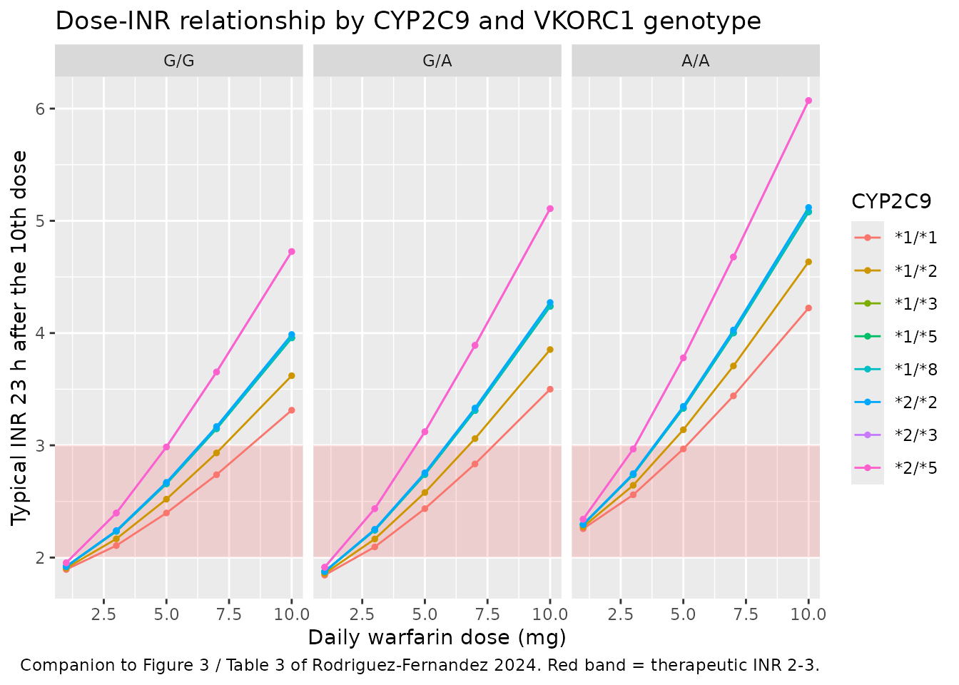
Validation 4 – probability of a therapeutic INR
The paper’s probability column comes from a 10,000-subject Monte Carlo simulation with log-normally distributed PD parameters. Reproduced here with 200 subjects per arm (the vignette cohort cap) for the 24 selected regimens.
N_PER_ARM <- 200

prob_subj <- published_t3 |>
  dplyr::select(cyp, vkorc1, dose_paper) |>
  dplyr::left_join(cyp_geno, by = "cyp") |>
  dplyr::left_join(vk_geno, by = "vkorc1") |>
  tidyr::crossing(rep = seq_len(N_PER_ARM)) |>
  dplyr::mutate(id = dplyr::row_number(), dose_mg = dose_paper) |>
  add_covariates()

prob_events <- make_events(prob_subj, "dose_mg", ii = 24, addl = 9L,
                           obs_times = sort(unique(c(seq(0, 240, by = 6), T_READ))))
stopifnot(!anyDuplicated(unique(prob_events[, c("id", "time", "evid")])))

probSim <- rxode2::rxSolve(mod, events = prob_events,
                           keep = c("cyp", "vkorc1", "dose_paper"),
                           returnType = "data.frame") |>
  dplyr::mutate(cyp = as.character(cyp), vkorc1 = as.character(vkorc1),
                dose_paper = as.numeric(as.character(dose_paper)))

prob_tab <- probSim |>
  dplyr::filter(abs(time - T_READ) < 1e-6) |>
  dplyr::group_by(cyp, vkorc1, dose_paper) |>
  dplyr::summarise(prob_model = 100 * mean(INR >= 2 & INR <= 3),
                   median_INR = median(INR), .groups = "drop") |>
  dplyr::left_join(published_t3, by = c("cyp", "vkorc1", "dose_paper")) |>
  dplyr::mutate(diff_pp = prob_model - prob_paper)
stopifnot(nrow(prob_tab) == 24L, !anyNA(prob_tab$prob_paper))

prob_tab |>
  dplyr::select(cyp, vkorc1, dose_paper, median_INR, prob_model, prob_paper, diff_pp) |>
  dplyr::rename(
    "CYP2C9"                  = cyp,
    "VKORC1"                  = vkorc1,
    "Dose (mg/d)"             = dose_paper,
    "Median INR at 239 h"     = median_INR,
    "P(INR 2-3) model (%)"    = prob_model,
    "P(INR 2-3) Table 3 (%)"  = prob_paper,
    "Difference (pp)"         = diff_pp
  ) |>
  knitr::kable(digits = 1, caption = paste(
    "Probability of a therapeutic INR at the Table 3 dose.",
    "200 subjects per arm here vs 10,000 in the paper."
))| CYP2C9 | VKORC1 | Dose (mg/d) | Median INR at 239 h | P(INR 2-3) model (%) | P(INR 2-3) Table 3 (%) | Difference (pp) |
|---|---|---|---|---|---|---|
| 1/1 | A/A | 3 | 2.6 | 61.0 | 67.0 | -6.0 |
| 1/1 | G/A | 5 | 2.4 | 68.0 | 66.7 | 1.3 |
| 1/1 | G/G | 5 | 2.5 | 75.5 | 66.2 | 9.3 |
| 1/2 | A/A | 3 | 2.7 | 62.5 | 64.7 | -2.2 |
| 1/2 | G/A | 5 | 2.7 | 64.0 | 67.3 | -3.3 |
| 1/2 | G/G | 5 | 2.6 | 71.0 | 69.2 | 1.8 |
| 1/3 | A/A | 3 | 2.9 | 54.0 | 64.6 | -10.6 |
| 1/3 | G/A | 3 | 2.3 | 61.0 | 60.7 | 0.3 |
| 1/3 | G/G | 5 | 2.7 | 59.0 | 65.9 | -6.9 |
| 1/5 | A/A | 3 | 2.9 | 52.0 | 60.6 | -8.6 |
| 1/5 | G/A | 5 | 2.9 | 52.0 | 63.6 | -11.6 |
| 1/5 | G/G | 5 | 2.8 | 56.5 | 65.2 | -8.7 |
| 1/8 | A/A | 3 | 2.9 | 53.5 | 63.5 | -10.0 |
| 1/8 | G/A | 5 | 2.8 | 57.5 | 62.4 | -4.9 |
| 1/8 | G/G | 5 | 2.7 | 63.5 | 63.6 | -0.1 |
| 2/2 | A/A | 1 | 2.3 | 63.0 | 60.8 | 2.2 |
| 2/2 | G/A | 5 | 2.8 | 59.0 | 62.5 | -3.5 |
| 2/2 | G/G | 5 | 2.7 | 52.0 | 63.5 | -11.5 |
| 2/3 | A/A | 1 | 2.4 | 70.0 | 64.3 | 5.7 |
| 2/3 | G/A | 3 | 2.5 | 65.5 | 63.0 | 2.5 |
| 2/3 | G/G | 3 | 2.4 | 67.0 | 64.9 | 2.1 |
| 2/5 | A/A | 1 | 2.3 | 63.0 | 63.2 | -0.2 |
| 2/5 | G/A | 3 | 2.5 | 64.5 | 67.3 | -2.8 |
| 2/5 | G/G | 3 | 2.4 | 66.5 | 62.4 | 4.1 |
# The paper's own claim is the one worth gating on: "the predicted probability
# in all scenarios reaches therapeutic INR levels in at least 60% of the
# patients" (Discussion), with a Table 3 range of 60.6-69.2%. With 200 subjects
# per arm the Monte Carlo standard error on a ~65% proportion is ~3.4 pp, so
# individual arms will scatter; assert on the CENTRE of the 24 arms, not on
# any single arm and not on the extremes.
stopifnot(
  # Structural: a mis-transcribed IC50, dose or IIV moves every arm's
  # probability by tens of points and breaks this instantly.
  abs(median(prob_tab$prob_model) - median(prob_tab$prob_paper)) < 12,
  # Envelope: robust to which subjects land in the tails.
  quantile(abs(prob_tab$diff_pp), 0.9) < 20,
  # The therapeutic window must be the modal outcome in every arm, which is
  # the qualitative claim Table 3 rests on.
  median(prob_tab$prob_model) > 45
)
probSim |>
  dplyr::mutate(vkorc1 = factor(vkorc1, levels = c("G/G", "G/A", "A/A"))) |>
  dplyr::group_by(time, vkorc1, cyp) |>
  dplyr::summarise(
    Q05 = quantile(INR, 0.05), Q50 = median(INR), Q95 = quantile(INR, 0.95),
    .groups = "drop"
  ) |>
  ggplot(aes(time / 24, Q50, colour = cyp, fill = cyp)) +
  annotate("rect", xmin = -Inf, xmax = Inf, ymin = 2, ymax = 3,
           fill = "red", alpha = 0.12) +
  geom_ribbon(aes(ymin = Q05, ymax = Q95), alpha = 0.12, colour = NA) +
  geom_line() +
  facet_wrap(~vkorc1) +
  labs(x = "Time (days)", y = "INR",
       colour = "CYP2C9", fill = "CYP2C9",
       title = "Simulated INR onset at the Table 3 dose for each genotype",
       caption = paste("Replicates Figure 3 of Rodriguez-Fernandez 2024",
                       "(median and 5th-95th percentiles, 200 subjects per arm).",
                       "Red band = therapeutic INR 2-3."))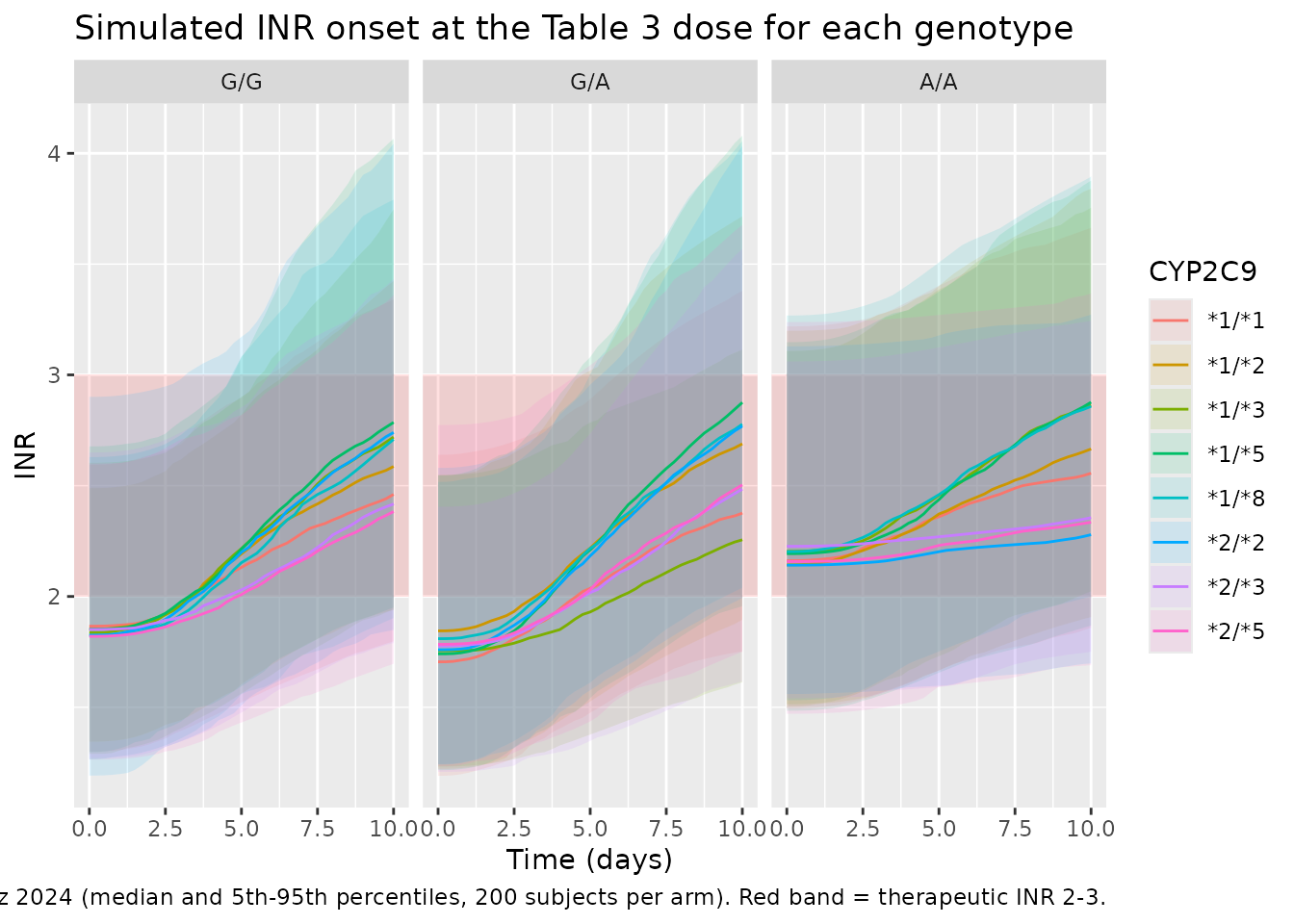
The slow onset visible here – INR is still climbing at day 10 – is a direct consequence of the fixed MTT2 of 110.9 h: the slow transit chain has a total transit time of 332.7 h (about 14 days), so 10 days of dosing does not reach the pharmacodynamic steady state. This is why the paper’s read-out time (23 h after the 10th dose) matters and is not interchangeable with a true steady-state INR.
Assumptions and deviations
-
The INR-response exponent is absent, and this was settled
numerically. The Hamberg models that Rodriguez-Fernandez 2024
builds on write the INR observation as
BASE + INRmax * (1 - A * B)^lambdawith an estimated exponentlambda(3.61 in Hamberg 2007). Table 2 of Rodriguez-Fernandez 2024 reports no such exponent, and the paper’s text never mentions one. The packaged model therefore useslambda = 1. This is not a guess: at the paper’s own IC50 values (9.22-11.76 mg/L, three to five times the European estimates), the steady-state warfarin concentration at a 1-10 mg daily dose produces only 1-7% inhibition, so1 - A * Bis of order 0.02-0.09. Withlambda = 3.61the maximum achievable INR across every genotype and every dose in Table 3 is 1.78-2.23 – essentially the baseline – so no dose could ever reach the therapeutic range and Table 3 could not exist. Withlambda = 2the same holds. Onlylambda = 1reproduces Table 3, and it reproduces all 24 of its dose selections (Validation 3). -
INRmaxis an additive increment above baseline, not an absolute ceiling. The paper says “the maximum INR was set to 20 as previously reported”; the Hamberg form it cites addsINRmaxto the subject’s baseline. At the small inhibition fractions this cohort operates at, the two readings differ by under 4% on the drug term, so the choice is not resolvable from the published numbers. The Hamberg form is used for consistency with the cited source. -
Transit-chain rate constant convention. The chains
use
ktr = 1 / MTT, matching the encoding ofmodellib("Hamberg_2007_warfarin_s"), whose MTT values Rodriguez-Fernandez 2024 fixes to. The paper states the chains have three compartments each but does not print the rate-constant definition. The choice affects the onset transient only, not the steady state, so Table 3 cannot discriminate betweenktr = 1/MTTandktr = n/MTT; the transient in the Figure 3 replicate above would be three times faster under the latter. -
Non-paper-derived parameter values: the entire PK
layer.
ka, the 0.14 L/kg volume and all six CYP2C9-diplotype elimination rate constants come from Reyes-Gonzalez 2020 (open access, PMC7892629), which Rodriguez-Fernandez 2024 fixes its PK to and cites as reference 20. No PK parameter value is printed anywhere in Rodriguez-Fernandez 2024 itself. Reyes-Gonzalez 2020 in turn tookkaand the volume from the literature and the elimination rate constants from its own reference 15; neither publication estimated them. -
CYP2C9 *3, *5, *6 and *8 are pooled. Reyes-Gonzalez
2020 defines a single reduced-function allele class “n” containing *3,
*5, *6 and *8, so *1/*3, *1/*5 and *1/*8 share one elimination rate
constant, as do *2/*3 and *2/*5. The model keeps the four allele-count
covariate columns separate and pools them inside
model(), so a future paper reporting allele-specific effects can reuse the same dataset. No *6 carriers were present in the cohort; the column is retained because the source model’s allele-class definition names *6. -
No PK residual error and no PK IIV. Warfarin
concentrations were never measured in this study, so there is nothing to
attach either to.
Ccis a deterministic function of genotype, weight and dose. -
Sex is not in the population metadata. The paper
describes the cohort as “mostly males” but publishes no sex breakdown,
so
sex_female_pctisNA. The authors note this as a study limitation. -
Screened-but-unretained covariates. Age, body
weight (on the PD parameters), CYP2C9 and VKORC1 (on parameters other
than those retained), race, diabetes mellitus and smoking status were
all tested univariately and none reached the p < 0.01 / 6.63-unit
dOFV threshold. No point estimates are published for them, so they are
recorded in the model file’s
covariatesDataExcludedlist as documentation only. - Supplementary material not available. Supplementary Table S1 holds the base (pre-covariate) PK/PD parameter estimates, which are superseded by the final estimates in Table 2 used here; the supplement is a Word document that was not available when this model was built. Nothing in the final model depends on it. Supplementary Figures S1-S5 are diagnostic plots (covariate distributions, GOF, NPDE, eta distributions) and carry no parameter values.
- Virtual cohorts use the cohort median weight (83 kg). The paper’s simulations do not state the weight distribution used; holding weight fixed isolates the genotype effect, which is what Table 3 is stratified on.
- Cohort size. The probability reproduction uses 200 subjects per arm against the paper’s 10,000, so individual arm probabilities carry a Monte Carlo standard error of roughly 3.4 percentage points.