Tiropramide (Jeong 2020)
Source:vignettes/articles/Jeong_2020_tiropramide.Rmd
Jeong_2020_tiropramide.RmdModel and source
- Citation: Jeong SH, Jang JH, Cho HY, Lee YB. Population Pharmacokinetic Analysis of Tiropramide in Healthy Korean Subjects. Pharmaceutics. 2020;12(4):374. doi:10.3390/pharmaceutics12040374
- Article: https://doi.org/10.3390/pharmaceutics12040374 (open access)
Population
Jeong et al. (2020) re-analysed the reference-formulation period of a randomised, single-dose, two-way crossover bioequivalence study of tiropramide 100 mg tablets in 24 healthy Korean men (Section 2.1). Age ranged from 19 to 29 years (median 23), body weight from 52.5 to 82.8 kg (median 66.8), and serum total protein from 6.7 to 8.3 g/dL (median 7.6; Table 1). Plasma was sampled pre-dose and at 0.33, 0.67, 1, 1.5, 2, 2.5, 3, 4, 6, 8 and 12 h after a fasted oral dose, giving 288 concentrations (Section 3.1) measured by column-switching semi-micro HPLC with an LLOQ of 2 ng/mL (Section 3.3). ABCB1, CYP2D6, OCT2 and PEPT1 genotypes were determined for every subject (Table 2) and screened as covariates, but none was retained.
The final model (Section 3.5, Figure 2, Equation 1) is one-compartment with first-order elimination. The oral dose enters “depot 1” and, after an absorption lag time, transfers to “depot 2” at the first absorption rate constant Ka1, from which it enters the central compartment at Ka2. Serum total protein enters CL/F and V/F as a linear effect centred at the 7.6 g/dL median. Inter-individual variability is exponential on all five structural parameters, and the residual error is additive on log-transformed concentrations. The model was estimated in Phoenix NLME 8.1 with FOCE-ELS.
rxode2::rxode2(readModelDb("Jeong_2020_tiropramide"))$population
#> ℹ parameter labels from comments will be replaced by 'label()'
#> $species
#> [1] "human"
#>
#> $n_subjects
#> [1] 24
#>
#> $n_studies
#> [1] 1
#>
#> $n_observations
#> [1] 288
#>
#> $age_range
#> [1] "19-29 years"
#>
#> $age_median
#> [1] "23 years"
#>
#> $weight_range
#> [1] "52.5-82.8 kg"
#>
#> $weight_median
#> [1] "66.8 kg"
#>
#> $sex_female_pct
#> [1] 0
#>
#> $race_ethnicity
#> Asian
#>   100
#>
#> $disease_state
#> [1] "healthy volunteers"
#>
#> $dose_range
#> [1] "100 mg single oral tablet (reference formulation of a two-way crossover bioequivalence study), fasted"
#>
#> $regions
#> [1] "Republic of Korea"
#>
#> $total_protein_range
#> [1] "6.7-8.3 g/dL (median 7.6)"
#>
#> $notes
#> [1] "Healthy Korean men from a randomized single-dose crossover bioequivalence study; only the reference-formulation period was analysed. Sampling 0-12 h. Demographics from Table 1; genotypes (ABCB1, CYP2D6, OCT2, PEPT1) in Table 2. Estimated in Phoenix NLME 8.1 (FOCE-ELS)."
Source trace
| Quantity | Value | Source location |
|---|---|---|
| Structure: depot 1 -> depot 2 -> central, lag on depot 1 | – | Section 3.5 text; Figure 2 schematic and caption |
| Covariate equations (linear, centred at 7.6 g/dL) | – | Equation 1 |
Ka1 (lktr) |
3.187 1/h | Table 6, final model, tvKa1 |
Ka2 (lka) |
3.183 1/h | Table 6, final model, tvKa2 |
V/F (lvc) |
1,889,250.002 mL = 1889.25 L | Table 6, final model, tvV/F |
CL/F (lcl) |
466,711.101 mL/h = 466.711 L/h | Table 6, final model, tvCL/F |
Tlag (ltlag) |
0.196 h | Table 6, final model, tvTlag |
Total protein on CL/F (e_tpro_cl) |
-0.804 per g/dL | Table 6, dCl/FdTotalproteins; sign confirmed by Table 7 |
Total protein on V/F (e_tpro_vc) |
-1.049 per g/dL | Table 6, dV/FdTotalproteins; sign confirmed by Table 7 |
| omega^2 Ka1 / Ka2 | 0.557 / 0.556 | Table 6, final model |
| omega^2 V/F / CL/F / Tlag | 0.326 / 0.160 / 0.107 | Table 6, final model |
sigma (expSd) |
0.357 | Table 6, final model; log-additive form in Section 2.6 |
| Dose, sampling times, LLOQ | 100 mg; 0-12 h; 2 ng/mL | Sections 2.1 and 3.3 |
The Table 6 IIV (%) column equals 100 * sqrt(omega^2)
(for example sqrt(0.326) = 0.571, printed as 57.118%),
which confirms that the omega column holds variances. The residual row
is printed as sigma (not sigma^2) alongside
omega^2 rows and is used as the log-scale standard
deviation.
Load the model
mod <- rxode2::rxode2(readModelDb("Jeong_2020_tiropramide"))
#> ℹ parameter labels from comments will be replaced by 'label()'
mod_typical <- rxode2::zeroRe(mod)
Typical-value checks
For a first-order-elimination model the area under the curve after a
single oral dose is exactly Dose / (CL/F), whatever the
absorption chain looks like, and the terminal half-life is
log(2) * V / CL because both absorption rate constants
(about 3.2 1/h) are much faster than elimination (CL/V =
0.247 1/h). At the median total protein of 7.6 g/dL (76 g/L) the
expected values are 100 mg / 466.711 L/h = 214.27 ng*h/mL
and log(2) * 1889.25 / 466.711 = 2.806 h.
obs_dense <- c(seq(0, 2, by = 0.02), seq(2.05, 72, by = 0.05))

ev_typ <- rxode2::et(amt = 100, cmt = "depot") |>
  rxode2::et(obs_dense, cmt = "central") |>
  as.data.frame()
ev_typ$TPRO <- 76

sim_typ <- as.data.frame(rxode2::rxSolve(mod_typical, events = ev_typ))
#> ℹ omega/sigma items treated as zero: 'etalktr', 'etalka', 'etalvc', 'etalcl', 'etaltlag'

auc_typ <- sum(diff(sim_typ$time) *
  (utils::head(sim_typ$Cc, -1) + utils::tail(sim_typ$Cc, -1)) / 2)
auc_expected <- 100 / 466.711101 * 1000

term <- sim_typ[sim_typ$time >= 24, ]
thalf_typ <- log(2) / -stats::coef(stats::lm(log(Cc) ~ time, data = term))[["time"]]
thalf_expected <- log(2) * 1889.250002 / 466.711101

c(
  auc_sim = auc_typ, auc_expected = auc_expected,
  thalf_sim = thalf_typ, thalf_expected = thalf_expected
)
#>        auc_sim   auc_expected      thalf_sim thalf_expected
#>     214.266401     214.265313       2.805865       2.805865

stopifnot(
  # Same drawn parameters on both sides (typical values): pure numerical error.
  abs(auc_typ / auc_expected - 1) < 0.01,
  abs(thalf_typ / thalf_expected - 1) < 0.01
)
The lag time delays the first appearance of drug in plasma: the
typical concentration is exactly zero until
Tlag = 0.196 h.
Total-protein effect
Equation 1 scales CL/F and V/F by
1 + (TP - 7.6) * slope. Across the observed total-protein
range (6.7-8.3 g/dL) this moves CL/F between 1.72-fold and 0.44-fold,
and V/F between 1.94-fold and 0.27-fold, of the median-subject value.
Higher total protein therefore means lower CL/F, lower V/F and higher
exposure, consistent with the negative correlations shown in Figure
3.
tp_grid <- c(6.7, 7.2, 7.6, 8.0, 8.3)
sim_tp <- dplyr::bind_rows(lapply(tp_grid, function(tp) {
  ev <- rxode2::et(amt = 100, cmt = "depot") |>
    rxode2::et(seq(0, 12, by = 0.05), cmt = "central") |>
    as.data.frame()
  ev$TPRO <- tp * 10
  as.data.frame(rxode2::rxSolve(mod_typical, events = ev)) |>
    dplyr::mutate(tp_gdL = tp)
}))
#> ℹ omega/sigma items treated as zero: 'etalktr', 'etalka', 'etalvc', 'etalcl', 'etaltlag'
#> ℹ omega/sigma items treated as zero: 'etalktr', 'etalka', 'etalvc', 'etalcl', 'etaltlag'
#> ℹ omega/sigma items treated as zero: 'etalktr', 'etalka', 'etalvc', 'etalcl', 'etaltlag'
#> ℹ omega/sigma items treated as zero: 'etalktr', 'etalka', 'etalvc', 'etalcl', 'etaltlag'
#> ℹ omega/sigma items treated as zero: 'etalktr', 'etalka', 'etalvc', 'etalcl', 'etaltlag'

ggplot(sim_tp, aes(time, Cc, colour = factor(tp_gdL))) +
  geom_line() +
  labs(
    x = "Time after dose (h)",
    y = "Tiropramide (ng/mL)",
    colour = "Total protein (g/dL)",
    title = "Typical profiles across the observed total-protein range, 100 mg"
  ) +
  theme_bw()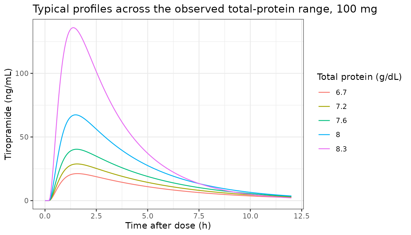
tp_auc <- sim_tp |>
  dplyr::group_by(tp_gdL) |>
  dplyr::summarise(
    auc_0_12 = sum(diff(time) * (utils::head(Cc, -1) + utils::tail(Cc, -1)) / 2),
    .groups = "drop"
  )
tp_auc |>
  dplyr::rename("Total protein (g/dL)" = tp_gdL, "AUC0-12 (ng*h/mL)" = auc_0_12) |>
knitr::kable(digits = 1)| Total protein (g/dL) | AUC0-12 (ng*h/mL) |
|---|---|
| 6.7 | 113.5 |
| 7.2 | 149.7 |
| 7.6 | 200.6 |
| 8.0 | 303.2 |
| 8.3 | 484.8 |
Virtual cohort
A cohort of 200 virtual healthy men receives a single 100 mg oral dose. Total protein is drawn from a normal distribution with the Table 1 mean and SD (7.59 +/- 0.41 g/dL), truncated to the observed 6.7-8.3 g/dL range (the linear covariate form becomes non-positive for V/F above 8.55 g/dL, so extrapolation is not supported). Observations follow the study’s sampling schedule.
rxode2::rxSetSeed(20200418)
set.seed(20200418)
n_sub <- 200
tp_draw <- numeric(0)
while (length(tp_draw) < n_sub) {
  x <- rnorm(n_sub, 7.59, 0.41)
  tp_draw <- c(tp_draw, x[x >= 6.7 & x <= 8.3])
}
cohort <- tibble::tibble(id = seq_len(n_sub), TPRO = tp_draw[seq_len(n_sub)] * 10)

samp_times <- c(0, 0.33, 0.67, 1, 1.5, 2, 2.5, 3, 4, 6, 8, 12)
ev_one <- rxode2::et(amt = 100, cmt = "depot") |>
  rxode2::et(sort(unique(c(samp_times, seq(0, 12, by = 0.1)))), cmt = "central") |>
  as.data.frame()

ev_all <- dplyr::bind_rows(lapply(seq_len(n_sub), function(i) {
  e <- ev_one
  e$id <- cohort$id[i]
  e$TPRO <- cohort$TPRO[i]
  e
}))

sim <- as.data.frame(rxode2::rxSolve(mod, events = ev_all, keep = "TPRO"))
Visual predictive check (Figure 5)
vpc <- sim |>
  dplyr::filter(time > 0) |>
  dplyr::group_by(time) |>
  dplyr::summarise(
    p05 = quantile(sim, 0.05),
    p50 = quantile(sim, 0.50),
    p95 = quantile(sim, 0.95),
    .groups = "drop"
  )

ggplot(vpc, aes(time)) +
  geom_ribbon(aes(ymin = p05, ymax = p95), fill = "steelblue", alpha = 0.25) +
  geom_line(aes(y = p50), colour = "steelblue") +
  geom_hline(yintercept = 2, linetype = "dotted") +
  scale_y_log10() +
  labs(
    x = "Time after dose (h)",
    y = "Tiropramide (ng/mL, log scale)",
    title = "Simulated median and 90% prediction interval, 100 mg single dose",
    caption = "Replicates the layout of Figure 5 of Jeong 2020. Dotted line: LLOQ 2 ng/mL."
  ) +
  theme_bw()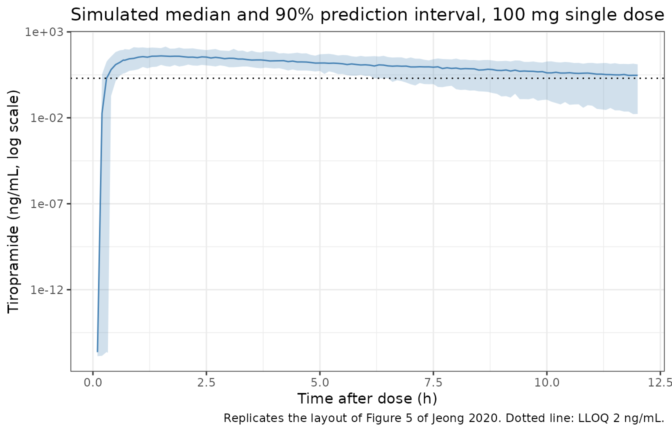
PKNCA validation
NCA is run per subject on the individual predictions
(Cc, without residual error) at the study’s sampling times,
with concentrations below the 2 ng/mL LLOQ removed, as they would have
been in the observed data.
nca_conc <- sim |>
  dplyr::filter(time %in% samp_times) |>
  dplyr::mutate(Cc = ifelse(time > 0 & Cc < 2, NA_real_, Cc)) |>
  dplyr::filter(!is.na(Cc)) |>
  dplyr::mutate(treatment = "100 mg oral") |>
  dplyr::select(id, time, Cc, treatment)

nca_dose <- cohort |>
  dplyr::transmute(id, time = 0, amt = 100, treatment = "100 mg oral")

conc_obj <- PKNCA::PKNCAconc(nca_conc, Cc ~ time | treatment + id,
  concu = "ng/mL", timeu = "h"
)
dose_obj <- PKNCA::PKNCAdose(nca_dose, amt ~ time | treatment + id,
  doseu = "mg", route = "extravascular"
)
intervals <- data.frame(
  start = 0, end = Inf,
  cmax = TRUE, tmax = TRUE, auclast = TRUE, aucinf.obs = TRUE, half.life = TRUE
)
nca_res <- suppressWarnings(PKNCA::pk.nca(
  PKNCA::PKNCAdata(conc_obj, dose_obj, intervals = intervals)
))
Jeong 2020 reports arithmetic means for the observed NCA (Section 3.4) and for the same parameters derived from the final population model’s individual predictions (Section 3.5), so the simulated per-subject values are also summarised by their arithmetic mean before comparison.
sim_means <- as.data.frame(nca_res$result) |>
  dplyr::filter(PPTESTCD %in% c("cmax", "tmax", "auclast", "aucinf.obs", "half.life")) |>
  dplyr::group_by(PPTESTCD) |>
  dplyr::summarise(PPORRES = mean(PPORRES, na.rm = TRUE), .groups = "drop")

sim_long <- dplyr::bind_rows(
  sim_means |> dplyr::mutate(comparison = "Observed NCA (Section 3.4)"),
  sim_means |> dplyr::mutate(comparison = "Final-model predictions (Section 3.5)")
)

published <- tibble::tribble(
  ~comparison,                              ~cmax, ~tmax, ~auclast, ~aucinf.obs, ~half.life,
  "Observed NCA (Section 3.4)",             69.07,  1.74,   254.31,      280.34,       3.41,
  "Final-model predictions (Section 3.5)",  54.89,  1.65,   242.73,      260.92,       2.73
)

cmp <- nlmixr2lib::ncaComparisonTable(
  simulated = sim_long,
  reference = published,
  by = "comparison",
  units = c(cmax = "ng/mL", tmax = "h", auclast = "ng*h/mL", aucinf.obs = "ng*h/mL", half.life = "h")
)
knitr::kable(cmp, caption = "Mean NCA parameters: simulated cohort vs Jeong 2020.")| NCA parameter | comparison | Reference | Simulated | % diff |
|---|---|---|---|---|
| Cmax (ng/mL) | Observed NCA (Section 3.4) | 69.1 | 49.5 | -28.3%* |
| Cmax (ng/mL) | Final-model predictions (Section 3.5) | 54.9 | 49.5 | -9.8% |
| Tmax (h) | Observed NCA (Section 3.4) | 1.74 | 1.73 | -0.7% |
| Tmax (h) | Final-model predictions (Section 3.5) | 1.65 | 1.73 | +4.7% |
| AUC0-∞ (obs) (ng*h/mL) | Observed NCA (Section 3.4) | 280 | 248 | -11.4% |
| AUC0-∞ (obs) (ng*h/mL) | Final-model predictions (Section 3.5) | 261 | 248 | -4.8% |
| AUClast (ng*h/mL) | Observed NCA (Section 3.4) | 254 | 213 | -16.3% |
| AUClast (ng*h/mL) | Final-model predictions (Section 3.5) | 243 | 213 | -12.3% |
| t½ (h) | Observed NCA (Section 3.4) | 3.41 | 3.51 | +2.8% |
| t½ (h) | Final-model predictions (Section 3.5) | 2.73 | 3.51 | +28.5%* |
sim_auc <- sim_means$PPORRES[sim_means$PPTESTCD == "auclast"]
sim_cmax <- sim_means$PPORRES[sim_means$PPTESTCD == "cmax"]
stopifnot(
  # A mis-transcribed CL/F, V/F or unit (mL vs L) moves these by far more.
  abs(sim_auc / 242.73 - 1) < 0.25,
  abs(sim_cmax / 54.89 - 1) < 0.35
)
Tmax, AUC and Cmax agree with the paper’s final-model-derived values within about 12%. Two rows exceed the 20% flag:
- Cmax against the observed NCA. The observed mean Cmax (69.07 +/- 59.74 ng/mL) is higher and far more variable than both the paper’s own model-derived value (54.89 +/- 46.18 ng/mL) and the simulation. It is driven by a few very high individual peaks (Figure 1; the two PEPT1 GC subjects averaged 181 ng/mL, Table 3). The simulation sits within 10% of the model-derived value, which is the like-for-like comparison.
-
Half-life against the model-derived value. The
typical-subject half-life is 2.81 h (checked exactly above), close to
the paper’s model-derived mean of 2.73 h. The simulated cohort mean is
higher (about 3.5 h) because independent log-normal IIV on V/F (omega^2
0.326) and CL/F (0.160) makes the mean of
log(2) * V / CLlarger than its typical value (a factor of aboutexp((0.326 + 0.160) / 2) = 1.28before the total-protein effect). The paper’s value was computed from the 24 subjects’ empirical Bayes estimates, which do not carry the full population variance. The simulated mean agrees with the observed NCA half-life (3.41 h) within 3%.
The AUClast values are slightly lower than the paper’s because the NCA uses the 12 h sampling schedule with concentrations below the 2 ng/mL LLOQ removed; AUC0-inf, which extrapolates the tail, is within 5% of the model-derived value.
Assumptions and deviations
-
Parameter naming. The paper’s Ka1 moves drug from
depot 1 to depot 2 and Ka2 from depot 2 to the central compartment
(Figure 2 caption). They are encoded as
lktr(a single transit step,depot -> transit1) andlka(transit1 -> central), respectively. The lag time is applied to the dosing compartment (alag(depot)), matching the caption’s “delay time for the drug to move from depot 1 to depot 2”. -
Covariate units. Total protein is supplied in the
canonical g/L (
TPRO); the model divides by 10 internally so that Equation 1’s g/dL slopes and 7.6 g/dL centring apply unchanged. - Sign of the total-protein slopes. The PDF prints both slopes as negative in Table 6 and Table 7 (-0.804 on CL/F, -1.049 on V/F), consistent with the negative correlations in Figure 3 and the Discussion (“higher total protein levels in the blood mean a smaller distribution … and a lower excretion”).
- Validity range. The linear form in Equation 1 is only valid within the observed total-protein range. V/F reaches zero at 8.55 g/dL and CL/F at 8.84 g/dL; the virtual cohort is therefore truncated to 6.7-8.3 g/dL.
-
Residual error. The Table 6
sigma= 0.357 is taken as the SD of the additive log-scale error (Cc ~ lnorm(expSd)), following the table’s convention of printing variances asomega^2and the residual assigma. - Unit conversion. Table 6 reports V/F in mL and CL/F in mL/h; these are converted to L and L/h and the concentration is scaled by 1000 to give ng/mL from a mg dose.
-
Screened covariates. BMI, ABCB1 (1236C>T,
2677G>T/A, 3435C>T), CYP2D6 (1/10), OCT2 808G>T and
PEPT1 1287G>C were tested (Table 5) but not retained; the tested ones
are documented in the model’s
covariatesDataExcludedmetadata. - Errata. No erratum or correction for doi:10.3390/pharmaceutics12040374 was found in Europe PMC (no comment/correction links on the record) as of 2026-09-26.