Nadroparin (Romano 2023) • nlmixr2lib

Model and source

mod <- readModelDb("Romano_2023_nadroparin")
ui <- rxode2::rxode(mod)
#> ℹ parameter labels from comments will be replaced by 'label()'

Citation: Romano LGR, Hunfeld NGM, Kruip MJHA, Endeman H, Preijers T. Population pharmacokinetics of nadroparin for thromboprophylaxis in COVID-19 intensive care unit patients. Br J Clin Pharmacol. 2023;89(5):1617-1628. doi:10.1111/bcp.15634
Article: https://doi.org/10.1111/bcp.15634
PubMed Central: https://www.ncbi.nlm.nih.gov/pmc/articles/PMC9878197/

Romano 2023 is a population pharmacokinetic analysis of nadroparin, a low-molecular-weight heparin, given as thromboprophylaxis (5700 IU subcutaneously twice daily) to critically ill COVID-19 patients in the intensive care unit. The model is fitted to plasma anti-Xa activity, so clearance and volume are apparent anti-Xa parameters (CL/F in mL/h, Vd/F in mL) and the observation is in IU/mL. The clinical question is which regimen best reaches the 0.3-0.7 IU/mL anti-Xa target measured 4 h after a dose; the paper’s answer is 5700 IU twice daily.

The final model is one-compartment with first-order absorption. Apparent clearance carries all of the inter-individual variability and five covariate effects – higher C-reactive protein, D-dimer and CKD-EPI eGFR raise it, and vasopressor and corticosteroid use lower it by 25.1% and 22.5%:

$CL_i = 2230 \left(\frac{CRP}{100}\right)^{0.182} \left(\frac{\text{D-dimer}}{10}\right)^{0.117} \left(\frac{GFR_{CKD\text{-}EPI}}{80}\right)^{0.368} 0.749^{\text{Vasopressors}} \, 0.775^{\text{Corticosteroids}} \, e^{\eta_i}$

with CRP in mg/L, D-dimer in mg/L and eGFR in mL/min/1.73 m^2. The control stream in the paper’s Appendix SA computes the eGFR inside the model from serum creatinine, age and sex with the 2009 CKD-EPI equation; the packaged model does the same, so it takes CREAT (umol/L), AGE and SEXF rather than a precomputed eGFR column.

Population

The modelling cohort is 65 critically ill adults with PCR-confirmed SARS-CoV-2 infection admitted to the Erasmus MC intensive care unit (Rotterdam, the Netherlands) between March 2020 and January 2021, who contributed 280 anti-Xa samples (21 below the 0.1 IU/mL limit of quantification). A further 25 patients (147 samples) formed an internal validation cohort. Modelling-cohort medians (Table 1): age 62 years, body weight 89 kg, CRP 76 mg/L, D-dimer 1.29 mg/L, CKD-EPI eGFR 94.4 mL/min/1.73 m^2; 87% were mechanically ventilated, 89% received vasopressors and 65% corticosteroids at the start of sampling. Sex and race are not tabulated.

Source trace

Model element	Value	Source
Structure: depot -> central, first-order absorption and elimination	one compartment	Results 3.2; Table 2 (ka, CL, Vd only); Appendix SA ADVAN5, K12 = KA, K20 = CL/V2
`lka`	log(0.276 1/h)	Table 2 final model; Appendix SA THETA(3)
`lcl`	log(2230 mL/h)	Table 2 final model and CL equation; Appendix SA THETA(4)
`lvc`	log(11 000 mL)	Table 2 final model; Appendix SA THETA(5)
`e_crp_cl`	0.182, (CRP/100)^theta	Table 2 ‘CL-CRP’; Appendix SA THETA(6), COV_CL
`e_ddimer_cl`	0.117, (D-dimer/10 mg/L)^theta	Table 2 ‘CL-D-dimer’; Appendix SA THETA(7), COV_DDMR; unit from Table 1 and Figure 5 axis
`e_inotrope_cl`	0.749^Vasopressors	Table 2 ‘CL-use of vasopressors’; Appendix SA THETA(8), COV_VASO
`e_crcl_cl`	0.368, (eGFR/80)^theta	Table 2 ‘CL-GFR CKD-EPI’; Appendix SA THETA(9), COV_CL2
`e_steroid_cl`	0.775^Corticosteroids	Table 2 ‘CL-use of corticosteroids’; Appendix SA THETA(10), COV_CORT
CKD-EPI 2009 eGFR	141, kappa 61.9 / 79.6 umol/L, alpha -0.329 / -0.411, -1.209, 0.993^AGE, x 1.018 female	Appendix SA $PK
`etalcl`	variance 0.115 (34.9% CV)	Appendix SA $OMEGA; Table 2 IIV on CL
`addSd`	0.0859 IU/mL	Appendix SA THETA(1); Table 2 0.086
`propSd`	0.2	Appendix SA THETA(2); Table 2 0.2
Error form	sqrt(add^2 + prop^2 IPRED^2)	Appendix SA $ERROR, W

Closed-form checks

The in-model eGFR reproduces the CKD-EPI 2009 equation

The egfr variable computed inside the model is compared with an independent evaluation of the 2009 CKD-EPI equation (creatinine converted from umol/L to mg/dL) for creatinine values on both sides of the sex-specific knot.

ckd_epi_2009 <- function(scr_umol, age, female) {
  scr <- scr_umol / 88.4
  kappa <- ifelse(female == 1, 0.7, 0.9)
  alpha <- ifelse(female == 1, -0.329, -0.411)
  141 * pmin(scr / kappa, 1)^alpha * pmax(scr / kappa, 1)^-1.209 *
    0.993^age * ifelse(female == 1, 1.018, 1)
}

egfr_grid <- tidyr::expand_grid(
  CREAT = c(40, 61.9, 70, 79.6, 120, 250),
  SEXF = c(0, 1)
) |>
  mutate(id = row_number(), AGE = 62, CRP = 100, DDIMER = 10000,
         CONMED_INOTROPE = 0, CONMED_STEROID = 0)

egfr_ev <- egfr_grid |>
  mutate(time = 0, amt = 0, evid = 0, cmt = "central") |>
  select(id, time, amt, evid, cmt, everything())

egfr_sim <- rxode2::rxSolve(rxode2::zeroRe(mod), egfr_ev, returnType = "data.frame")
#> ℹ parameter labels from comments will be replaced by 'label()'
#> ℹ omega/sigma items treated as zero: 'etalcl'
#> Warning: multi-subject simulation without without 'omega'
egfr_chk <- egfr_grid |>
  mutate(egfr_model = egfr_sim$egfr,
         egfr_closed = ckd_epi_2009(CREAT, AGE, SEXF))

knitr::kable(egfr_chk |> select(CREAT, SEXF, egfr_model, egfr_closed), digits = 2)

CREAT	SEXF	egfr_model	egfr_closed
40.0	0	121.03	121.01
40.0	1	107.20	107.19
61.9	0	101.15	101.13
61.9	1	92.86	92.82
70.0	0	96.16	96.14
70.0	1	80.03	80.00
79.6	0	91.22	91.16
79.6	1	68.51	68.49
120.0	0	55.53	55.50
120.0	1	41.71	41.69
250.0	0	22.86	22.85
250.0	1	17.17	17.17

# Same equation evaluated twice: the only difference is the umol/L kappa
# rounding (61.9 and 79.6 vs 0.7 * 88.4 and 0.9 * 88.4).
stopifnot(all(abs(egfr_chk$egfr_model / egfr_chk$egfr_closed - 1) < 0.002))

Typical clearance at the reference patient

Romano 2023 Table 2 states the typical values hold for a patient with CRP 100 mg/L, D-dimer 10 mg/L and eGFR 80 mL/min/1.73 m^2 on neither corticosteroids nor vasopressors. With the creatinine back-calculated to give an eGFR of exactly 80, the model’s typical clearance must be 2230 mL/h.

# Inverts the CKD-EPI 2009 equation for creatinine (umol/L).
ckd_epi_2009_creat <- function(egfr, age, female) {
  kappa <- ifelse(female == 1, 61.9, 79.6)
  alpha <- ifelse(female == 1, -0.329, -0.411)
  r <- egfr / (141 * 0.993^age * ifelse(female == 1, 1.018, 1))
  kappa * ifelse(r >= 1, r^(1 / alpha), r^(-1 / 1.209))
}

ref_ev <- data.frame(
  id = 1, time = 0, amt = 0, evid = 0, cmt = "central",
  CRP = 100, DDIMER = 10000, AGE = 62, SEXF = 0,
  CREAT = ckd_epi_2009_creat(80, 62, 0),
  CONMED_INOTROPE = 0, CONMED_STEROID = 0
)
ref_sim <- rxode2::rxSolve(rxode2::zeroRe(mod), ref_ev, returnType = "data.frame")
#> ℹ parameter labels from comments will be replaced by 'label()'
#> ℹ omega/sigma items treated as zero: 'etalcl'
c(egfr = ref_sim$egfr, cl_mL_h = ref_sim$cl)
#>    egfr cl_mL_h 
#>      80    2230
stopifnot(abs(ref_sim$egfr - 80) < 1e-6, abs(ref_sim$cl - 2230) < 1e-6)

The D-dimer reference is 10 mg/L

The D-dimer reference of 10 sits at the top of the observed range (Table 1 median 1.24 mg/L), which is unusual enough to check. Figure 5 plots D-dimer on a 0-10 mg/L axis, and a second, independent check comes from the structural model: before covariates were added, Romano 2023 estimated a population clearance of 1140 mL/h (Table 2, structural model). Evaluating the final model at the modelling-cohort median covariates, with each binary effect weighted by its prevalence (the geometric mean of the factor across the cohort), should land near that value if D-dimer is read in mg/L. Reading the reference as the cohort median instead would move clearance by a factor of (10 / 1.29)^0.117 = 1.27.

theta <- ui$theta
cl_median_patient <- unname(
  exp(theta["lcl"]) *
    (76 / 100)^theta["e_crp_cl"] *
    (1.29 / 10)^theta["e_ddimer_cl"] *
    (94.4 / 80)^theta["e_crcl_cl"] *
    theta["e_inotrope_cl"]^0.89 *
    theta["e_steroid_cl"]^0.65
)
c(final_model_at_median = cl_median_patient, structural_model = 1140)
#> final_model_at_median      structural_model 
#>              1162.357              1140.000
stopifnot(abs(cl_median_patient / 1140 - 1) < 0.05)

The simulated steady state matches the closed form

ss_closed <- function(dose, tau, t, cl, v, ka) {
  k <- cl / v
  dose * ka / (v * (ka - k)) *
    (exp(-k * t) / (1 - exp(-k * tau)) - exp(-ka * t) / (1 - exp(-ka * tau)))
}

cf_ev <- data.frame(
  id = 1, time = c(0, 240 + 4), amt = c(5700, 0), evid = c(1, 0),
  cmt = c("depot", "central"), ii = c(12, 0), addl = c(20, 0),
  CRP = 100, DDIMER = 10000, AGE = 62, SEXF = 0,
  CREAT = ckd_epi_2009_creat(80, 62, 0),
  CONMED_INOTROPE = 0, CONMED_STEROID = 0
)
cf_sim <- rxode2::rxSolve(rxode2::zeroRe(mod), cf_ev, returnType = "data.frame")
#> ℹ parameter labels from comments will be replaced by 'label()'
#> ℹ omega/sigma items treated as zero: 'etalcl'
cf_ref <- ss_closed(5700, 12, 4, 2230, 11000, 0.276)
c(simulated = cf_sim$Cc[cf_sim$time == 244], closed_form = cf_ref)
#>   simulated closed_form 
#>   0.2794079   0.2794081
# Same parameters on both sides: the difference is solver tolerance and the
# residual distance from steady state after 20 doses (k * 240 h = 48.7).
stopifnot(abs(cf_sim$Cc[cf_sim$time == 244] / cf_ref - 1) < 1e-4)

Virtual cohort

The cohort reproduces the modelling-cohort covariate distributions in Table 1. CRP, D-dimer and eGFR are drawn log-normally from their medians and interquartile ranges, age normally, and the two medication indicators as Bernoulli draws at the Table 1 prevalences. The paper does not tabulate sex, so 70% of patients are assumed male; serum creatinine is then back-calculated from the drawn eGFR, age and sex, so the eGFR the model computes reproduces the drawn value exactly. Covariates are held constant within a patient.

rxode2::rxSetSeed(20230501)
n_per_arm <- 200

lnorm_from_iqr <- function(n, median, q1, q3) {
  exp(rnorm(n, log(median), (log(q3) - log(q1)) / (2 * qnorm(0.75))))
}

cohort <- tibble(
  pid = seq_len(n_per_arm),
  AGE = pmin(pmax(rnorm(n_per_arm, 62, (70 - 53) / (2 * qnorm(0.75))), 25), 85),
  SEXF = rbinom(n_per_arm, 1, 0.30),
  CRP = lnorm_from_iqr(n_per_arm, 76.0, 35.5, 124),
  DDIMER = 1000 * lnorm_from_iqr(n_per_arm, 1.29, 0.87, 2.19),
  egfr_target = pmin(lnorm_from_iqr(n_per_arm, 94.4, 78.6, 111), 160),
  CONMED_INOTROPE = rbinom(n_per_arm, 1, 0.89),
  CONMED_STEROID = rbinom(n_per_arm, 1, 0.65)
) |>
  mutate(CREAT = ckd_epi_2009_creat(egfr_target, AGE, SEXF))

cohort |>
  summarise(across(c(AGE, CRP, DDIMER, egfr_target, CREAT), median),
            vasopressor = mean(CONMED_INOTROPE), corticosteroid = mean(CONMED_STEROID),
            female = mean(SEXF)) |>
  knitr::kable(digits = 2)

AGE	CRP	DDIMER	egfr_target	CREAT	vasopressor	corticosteroid	female
63.45	69.83	1175.73	94.72	66.89	0.88	0.66	0.3

Simulation of the dosing regimens in Figure 4

Each patient receives each of the four regimens Romano 2023 compares (3800 IU, 5700 IU and 7600 IU twice daily, 5700 IU once daily) for ten days, long enough to be at steady state (the elimination half-life is about 7 h for a patient at the cohort-median covariates and 3.4 h at the reference patient). The last dosing interval is sampled densely.

regimens <- tibble(
  regimen = c("3800 IU BID", "5700 IU BID", "7600 IU BID", "5700 IU QD"),
  dose = c(3800, 5700, 7600, 5700),
  tau = c(12, 12, 12, 24)
) |>
  mutate(n_dose = 240 / tau, t_last = 240 - tau)

arms <- tidyr::crossing(regimens, cohort) |>
  mutate(id = row_number())

dose_rows <- arms |>
  transmute(id, time = 0, amt = dose, evid = 1, cmt = "depot",
            ii = tau, addl = n_dose - 1)
obs_rows <- arms |>
  select(id, t_last, tau) |>
  tidyr::crossing(tad = seq(0, 24, by = 0.25)) |>
  filter(tad <= tau) |>
  transmute(id, time = t_last + tad, amt = 0, evid = 0, cmt = "central",
            ii = 0, addl = 0)

events <- bind_rows(dose_rows, obs_rows) |>
  left_join(arms |> select(id, regimen, AGE, SEXF, CRP, DDIMER, CREAT,
                           CONMED_INOTROPE, CONMED_STEROID), by = "id") |>
  arrange(id, time, desc(evid)) |>
  select(id, time, amt, evid, cmt, ii, addl, everything())

sim <- rxode2::rxSolve(mod, events |> select(-regimen), returnType = "data.frame") |>
  left_join(arms |> select(id, regimen, t_last), by = "id") |>
  mutate(tad = time - t_last)
#> ℹ parameter labels from comments will be replaced by 'label()'

Steady-state anti-Xa 4 h and 12 h after a dose (Figure 4)

Figure 4 of Romano 2023 shows, for the modelling cohort, the steady-state anti-Xa activity 4 h after a dose computed from each patient’s empirical Bayes clearance. The digitised medians are compared with the simulated individual predictions (Cc, which carries the clearance random effect but not residual error) at the same times.

at_times <- sim |>
  filter(tad %in% c(4, 12)) |>
  mutate(regimen = factor(regimen, levels = regimens$regimen))

ggplot(at_times |> filter(tad == 4), aes(regimen, Cc)) +
  geom_boxplot(outlier.size = 0.8) +
  geom_hline(yintercept = c(0.3, 0.7), linetype = "dashed", colour = "darkgreen") +
  labs(x = NULL, y = "Steady-state anti-Xa at t = 4 h (IU/mL)",
       caption = "Replicates Figure 4 (modelling cohort, t = 4 h) of Romano 2023.")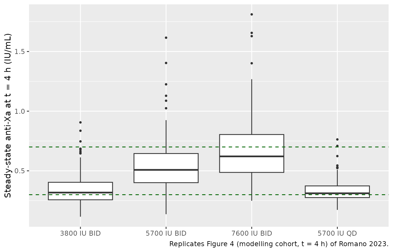

fig4 <- tribble(
  ~regimen, ~tad, ~published_median, ~published_pct_in_range,
  "3800 IU BID", 4, 0.30, 46.2,
  "5700 IU BID", 4, 0.45, 55.4,
  "7600 IU BID", 4, 0.60, 52.3,
  "5700 IU QD", 4, 0.31, 52.3,
  "5700 IU BID", 12, 0.27, NA,
  "7600 IU BID", 12, 0.36, NA
)

fig4_cmp <- at_times |>
  group_by(regimen, tad) |>
  summarise(simulated_median = median(Cc),
            simulated_pct_in_range = 100 * mean(Cc >= 0.3 & Cc <= 0.7),
            .groups = "drop") |>
  mutate(regimen = as.character(regimen)) |>
  inner_join(fig4, by = c("regimen", "tad")) |>
  mutate(pct_diff_median = 100 * (simulated_median / published_median - 1))

fig4_cmp |>
  select(regimen, tad, published_median, simulated_median, pct_diff_median,
         published_pct_in_range, simulated_pct_in_range) |>
  dplyr::rename(
    "Regimen" = regimen, "Time after dose (h)" = tad,
    "Figure 4 median (IU/mL)" = published_median,
    "Simulated median (IU/mL)" = simulated_median,
    "Median difference (%)" = pct_diff_median,
    "Figure 4 % in 0.3-0.7" = published_pct_in_range,
    "Simulated % in 0.3-0.7" = simulated_pct_in_range
  ) |>
  knitr::kable(digits = c(0, 0, 2, 2, 1, 1, 1))

Regimen	Time after dose (h)	Figure 4 median (IU/mL)	Simulated median (IU/mL)	Median difference (%)	Figure 4 % in 0.3-0.7	Simulated % in 0.3-0.7
3800 IU BID	4	0.30	0.32	5.9	46.2	53.0
5700 IU BID	4	0.45	0.51	12.9	55.4	81.0
5700 IU BID	12	0.27	0.33	21.3	NA	52.5
7600 IU BID	4	0.60	0.62	3.5	52.3	61.5
7600 IU BID	12	0.36	0.38	6.1	NA	47.0
5700 IU QD	4	0.31	0.31	0.6	52.3	56.5


# Robust centre check: a mis-transcribed clearance, volume or covariate
# reference moves every regimen's median by tens of percent.
stopifnot(
  abs(median(fig4_cmp$pct_diff_median)) < 10,
  all(abs(fig4_cmp$pct_diff_median) < 25)
)

The simulated medians agree with the digitised Figure 4 medians. The fraction of patients inside the target range is reported but not asserted on: Figure 4 is built from empirical Bayes estimates, which shrink toward the typical value (14% shrinkage on clearance), and the observed cohort’s covariate joint distribution is not reproduced exactly by the independent draws above, so the tails – and hence the in-range fraction – differ more than the centre does.

Profile over a steady-state dosing interval (cf. Figure 2)

Figure 2 is a prediction-corrected visual predictive check against time after dose for the observed data, which mix first and later doses. The plot below shows the simulated 5700 IU twice-daily steady-state interval with residual error (sim), the observable that the visual predictive check compares with the data. The observed median in Figure 2 peaks near 0.43 IU/mL around 4 h after the dose.

sim |>
  filter(regimen == "5700 IU BID") |>
  group_by(tad) |>
  summarise(p05 = quantile(sim, 0.05), p50 = quantile(sim, 0.5),
            p95 = quantile(sim, 0.95), .groups = "drop") |>
  ggplot(aes(tad)) +
  geom_ribbon(aes(ymin = p05, ymax = p95), fill = "steelblue", alpha = 0.3) +
  geom_line(aes(y = p50), colour = "steelblue4") +
  geom_hline(yintercept = c(0.3, 0.7), linetype = "dashed", colour = "darkgreen") +
  labs(x = "Time after dose (h)", y = "Anti-Xa (IU/mL)",
       caption = "Median and 90% interval, 5700 IU BID at steady state; compare Figure 2 of Romano 2023.")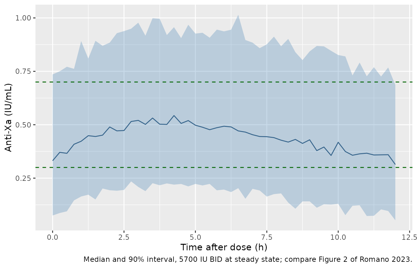

PKNCA validation

Non-compartmental analysis of the steady-state dosing interval, grouped by regimen. Romano 2023 reports no NCA, so the check is internal: at steady state the area over one dosing interval equals dose / CL for each patient.

nca_conc <- sim |>
  filter(!is.na(Cc)) |>
  select(id, regimen, tad, Cc)

nca_dose <- arms |>
  transmute(id, regimen, tad = 0, dose)

conc_obj <- PKNCA::PKNCAconc(nca_conc, Cc ~ tad | regimen + id)
dose_obj <- PKNCA::PKNCAdose(nca_dose, dose ~ tad | regimen + id)

intervals <- regimens |>
  transmute(regimen, start = 0, end = tau, cmax = TRUE, tmax = TRUE,
            auclast = TRUE, cmin = TRUE, cav = TRUE)

nca_res <- PKNCA::pk.nca(PKNCA::PKNCAdata(conc_obj, dose_obj, intervals = intervals))

nca_summary <- as.data.frame(nca_res) |>
  filter(PPTESTCD %in% c("cmax", "tmax", "auclast", "cmin", "cav")) |>
  group_by(regimen, PPTESTCD) |>
  summarise(median = median(PPORRES), .groups = "drop") |>
  tidyr::pivot_wider(names_from = PPTESTCD, values_from = median)

nca_summary |>
  dplyr::rename(
    "Regimen" = regimen, "Cmax (IU/mL)" = cmax, "Tmax (h)" = tmax,
    "AUCtau (IU*h/mL)" = auclast, "Cmin (IU/mL)" = cmin, "Cav (IU/mL)" = cav
  ) |>
  knitr::kable(digits = 3)

Regimen	AUCtau (IU*h/mL)	Cav (IU/mL)	Cmax (IU/mL)	Cmin (IU/mL)	Tmax (h)
3800 IU BID	3.267	0.272	0.318	0.198	4
5700 IU BID	5.279	0.440	0.508	0.327	4
5700 IU QD	4.717	0.197	0.319	0.065	5
7600 IU BID	6.362	0.530	0.621	0.382	4

auc_chk <- as.data.frame(nca_res) |>
  filter(PPTESTCD == "auclast") |>
  select(id, regimen, auclast = PPORRES) |>
  left_join(sim |> distinct(id, cl), by = "id") |>
  left_join(arms |> select(id, dose), by = "id") |>
  mutate(pct_diff = 100 * (auclast / (dose / cl) - 1))
summary(auc_chk$pct_diff)
#>      Min.   1st Qu.    Median      Mean   3rd Qu.      Max. 
#> -0.144191 -0.022629 -0.016779 -0.018930 -0.012495 -0.008268
# Same drawn clearance on both sides; the residual is trapezoidal error on a
# 15-min grid plus, for the slowest-clearing patients, a small shortfall from
# full steady state after ten days.
stopifnot(
  abs(median(auc_chk$pct_diff)) < 0.5,
  quantile(abs(auc_chk$pct_diff), 0.9) < 2
)

Assumptions and deviations

Sex distribution. Table 1 does not report sex. The virtual cohort assumes 70% male; sex enters the model only through the CKD-EPI eGFR, and because creatinine is back-calculated from the drawn eGFR the assumption does not change any simulated clearance.
Creatinine. Table 1 reports eGFR but not serum creatinine. The cohort draws eGFR from its Table 1 median and interquartile range and inverts the CKD-EPI equation for creatinine.
Covariate distributions. CRP, D-dimer and eGFR are drawn independently (log-normal from Table 1 medians and IQRs); the paper reports no collinearity among the retained covariates (Figure S2). Covariates are held constant within a patient, whereas the source data were time-varying.
Missing-covariate imputation. The Appendix SA control stream replaces a CRP of 0 (missing) by 100 mg/L and a missing eGFR by 80 mL/min/1.73 m^2. Its eGFR branch tests a variable GFR that is neither a data column nor defined in the code shown; because the eGFR exponent was estimated with a 33% RSE, the published run must have computed eGFR from creatinine, which is what the packaged model does. Neither imputation rule is part of the packaged model; supply observed values.
Baseline term. The control stream writes IPRED = F + BL with BL = TVBL, but TVBL is never defined and Results 3.2 states that a baseline parameter was not evaluated. The packaged model has no baseline.
Unused peripheral compartment. Appendix SA declares a PERIPH compartment under ADVAN5 but defines no rate constants for it, and Table 2 reports no intercompartmental clearance or peripheral volume; the model is one-compartment.
Below-quantification data. The paper fitted samples below 0.1 IU/mL with the M3 likelihood. That is an estimation device; simulations from the packaged model return uncensored values.
D-dimer units. The canonical DDIMER column is in ng/mL; the source recorded mg/L, so the model divides by 10000 ng/mL (the paper’s 10 mg/L reference). The structural-model check above supports the mg/L reading.
Figures 5 and 6 (Monte Carlo covariate scenarios) are not replicated: the paper draws covariates uniformly between unreported minima and maxima and does not state how the binary indicators were sampled.
No erratum was found for Romano 2023 (EuropePMC search, 2026-10-11).