Tebipenem (Ganesan 2023)
Source:vignettes/articles/Ganesan_2023_tebipenem.Rmd
Ganesan_2023_tebipenem.RmdModel and source
- Citation: Ganesan H, Gupta VK, Safir MC, Bhavnani SM, Talley AK, Melnick D, Rubino CM. Population Pharmacokinetic Analyses for Tebipenem after Oral Administration of Pro-Drug Tebipenem Pivoxil Hydrobromide. Antimicrob Agents Chemother. 2023 Jun 15;67(6):e0145122. doi:10.1128/aac.01451-22.
- Description: Two-compartment population PK model with two absorption transit compartments for tebipenem, the active moiety of the oral carbapenem pro-drug tebipenem pivoxil hydrobromide (TBP-PI-HBr), pooled across three phase 1 studies and the phase 3 ADAPT-PO trial in adults with complicated urinary tract infection / acute pyelonephritis (Ganesan 2023; 746 subjects, 3448 plasma concentrations). Apparent oral clearance is split into an additive non-renal arm (power function of creatinine clearance) and a renal arm (sigmoidal Hill function of creatinine clearance) that drives a cumulative urine compartment; the summed CL/F carries a linear body-surface-area effect. Central volume scales with height and peripheral volume with body surface area, both shifted by infection status. The absorption rate constant switches on fed status, is shifted by infection status, and carries a dose effect confined to the crossover thorough-QT study (study 104). Interindividual variability on CL/F is cohort-specific (healthy subjects vs infected patients) and Ka carries both IIV and two-occasion interoccasion variability.
- Article: https://doi.org/10.1128/aac.01451-22
- Supplement (Table S1, Figures S1-S6): https://doi.org/10.1128/aac.01451-22
Tebipenem pivoxil hydrobromide (TBP-PI-HBr) is an oral carbapenem pro-drug that is converted to the active moiety tebipenem in the enterocytes. Ganesan 2023 pooled three phase 1 studies with the phase 3 ADAPT-PO trial to build a population PK model for tebipenem intended for subsequent PK-PD target-attainment work.
Population
The final analysis data set comprised 746 subjects contributing 3,448 plasma concentrations (Ganesan 2023 Table 1). Of these, 99 were phase 1 subjects – 36 healthy adults from the single/multiple-ascending-dose study SPR994-101, 39 adults spanning normal renal function through end-stage renal disease from the renal-impairment study SPR994-102, and 24 healthy adults from the four-way-crossover thorough-QT study SPR994-104 – and 647 were patients with complicated urinary tract infection or acute pyelonephritis from ADAPT-PO (SPR994-301). Urine concentrations were additionally available from 67 phase 1 subjects and 37 phase 3 patients and are what make the renal clearance arm identifiable.
Pooled baseline characteristics were: age 60.0 years (18-91), height 169 cm (110-202), weight 76.0 kg (42.0-142), body surface area 1.86 m^2 (1.32-2.70), body mass index 26.3 kg/m^2 (15.3-57.9), and Cockcroft-Gault creatinine clearance normalized to body surface area 74.2 mL/min/1.73 m^2 (6.90-192). The population was 51.3% female and predominantly White (95.9% overall, 98.6% in ADAPT-PO), which is why race was tested but not retained as a covariate.
The same information is available programmatically from the model’s
population metadata
(readModelDb("Ganesan_2023_tebipenem")()$population).
pop <- readModelDb("Ganesan_2023_tebipenem")()$population
#> Warning: some etas defaulted to non-mu referenced, possible parsing error: etalcl_patient, etaiov_ka_1, etaiov_ka_2
#> as a work-around try putting the mu-referenced expression on a simple line
str(pop[c("n_subjects", "n_studies", "age_median", "bsa_median", "renal_function")])
#> List of 5
#>  $ n_subjects    : int 746
#>  $ n_studies     : int 4
#>  $ age_median    : chr "60.0 years"
#>  $ bsa_median    : chr "1.86 m^2"
#>  $ renal_function: chr "Creatinine clearance (Cockcroft-Gault, BSA-normalized) median 74.2 mL/min/1.73 m^2, range 6.90-192. Study 102 e"| __truncated__
Structural model
Ganesan 2023 supplemental Figure S3 gives the structure: an oral dose
enters a depot, passes through two transit compartments, and arrives in
a two-compartment disposition model. Every transfer along the absorption
chain is governed by the same rate constant Ka. Elimination
from the central compartment is split into two parallel first-order arms
– a non-renal arm and a renal arm – and the renal arm alone feeds the
cumulative urine compartment.
The transit chain replaced a lag-time-plus-first-order model: the two gave comparable fits to the dense phase 1 data, but the transit form was expected to converge more reliably against the sparse phase 3 sampling.
Source trace
Every ini() entry in
inst/modeldb/specificDrugs/Ganesan_2023_tebipenem.R carries
an in-file comment naming its origin. The table below collects them.
| Equation / parameter | Value | Source location |
|---|---|---|
| Structure (depot + 2 transit + 2-compartment + urine) | n/a | Supplemental Figure S3; Results “Population PK model development” |
lka (fasted) |
3.04 1/h | Eq. 6 coefficient on FAST; Table 2 row labelled “Ka
(fed)” (see Errata) |
e_fed_ka |
1.23 / 3.04 - 1 | Eq. 6 coefficient on (1 - FAST) = 1.23 1/h; Table 2 row
labelled “Ka (fasted)” |
e_healthy_ka |
0.368 | Table 2 “Ka:Infection status”; Eq. 6 |
e_dose_ka |
-0.478 | Table 2 “Ka:Dose effect”; Eq. 6 |
lcl_nonren |
15.6 L/h | Table 2 “CL NR” (Eq. 1 prints 10.2; see Errata) |
e_crcl_cl_nonren |
0.722 | Table 2 “CL NR, CLcr power”; Eq. 1 |
lcl_renal |
21.1 L/h | Table 2 “CL R, MAX”; Eq. 2 |
crcl50_cl_renal |
44.7 mL/min/1.73 m^2 | Table 2 “CL R, CLcr 50”; Eq. 2 |
hill_cl_renal |
2.13 | Table 2 “CL R, Hill”; Eq. 2 |
e_bsa_cl |
0.479 per m^2 | Table 2 “CL/F:BSA (slope)”; Eq. 3 |
lvc |
38.5 L | Table 2 “Vc/F”; Eq. 4 |
e_ht_vc |
2.09 | Table 2 “Vc/F:HTCM (power)”; Eq. 4 |
e_healthy_vc |
-0.290 | Table 2 “Vc/F:Infection status”; Eq. 4 |
lq |
2.23 L/h | Table 2 “CLd/F” |
lvp |
4.84 L | Table 2 “Vp/F”; Eq. 5 |
e_bsa_vp |
0.491 per m^2 | Table 2 “Vp/F:BSA (slope)”; Eq. 5 |
e_healthy_vp |
-0.245 | Table 2 “Vp/F:Infection status”; Eq. 5 |
etalcl_healthy |
0.0614 | Table 2 “IIV CL (phase 1)” |
etalcl_patient |
0.328 | Table 2 “IIV CL (phase 3)” |
etalvc |
0.197 | Table 2 “IIV Vc/F” |
etalvp |
0.0115 | Table 2 “IIV Vp/F” |
etalka |
0.518 | Table 2 “IIV Ka” |
etaiov_ka_1, etaiov_ka_2
|
0.201 | Table 2 “IOV Ka (Occ. 1)” / “(Occ. 2)” |
propSd |
sqrt(0.209) = 0.457 | Table 2 “RV prop, plasma” |
propSd_urineAmt |
sqrt(0.298) = 0.546 | Table 2 “RV prop, urine” |
| Reference CRCL 79.32, BSA 1.86, HT 169, dose 1200 mg | n/a | Eq. 1, Eq. 3 / Eq. 5, Eq. 4, Eq. 6 |
| Baseline demographics | n/a | Table 1 |
| Published exposure summary used below | n/a | Table 3 |
Note that Ganesan 2023 reports the interindividual and interoccasion
terms as variances with the corresponding %CV in parentheses computed as
sqrt(omega^2) (0.0614 -> 24.8 %CV, 0.518 -> 71.9
%CV), so the tabulated numbers are used directly as variances with no
log(CV^2 + 1) back-transform. The residual-variability rows
are likewise variances whose parenthetical values are the corresponding
standard deviations, and it is the standard deviations that the model
file carries.
Renal function and clearance (replicates Figure 4)
The most clinically consequential covariate is renal function.
Apparent oral clearance is the sum of a non-renal arm that is a power
function of creatinine clearance and a renal arm that is a sigmoidal
Hill function of it, with the sum scaled by a linear body-surface-area
term (Eq. 1-3). The curve below is extracted from the packaged model
itself – the clearance terms are read out of the rxSolve()
output rather than recomputed in R – so it tests the encoding rather
than restating it.
mod <- readModelDb("Ganesan_2023_tebipenem")

crcl_grid <- seq(7, 195, by = 1)

grid_events <- tibble(
  id               = seq_along(crcl_grid),
  CRCL             = crcl_grid,
  BSA              = 1.86,
  HT               = 169,
  DIS_HEALTHY      = 0,
  FED              = 0,
  DOSE_TBPPI_MG    = 600,
  STUDY_SPR994_104 = 0,
  OCC              = 1
) |>
  tidyr::crossing(time = c(0, 1)) |>
  mutate(amt = NA_real_, evid = 0L, cmt = "central", dvid = 1L)

sim_grid <-
  rxode2::rxSolve(
    mod,
    events    = grid_events,
    omega     = NA,
    keep      = c("CRCL", "BSA", "HT"),
    useLinCmt = FALSE
  ) |>
  as.data.frame() |>
  filter(time == 1) |>
  mutate(clf = cl_nonren + cl_renal)
#> ℹ parameter labels from comments will be replaced by 'label()'
#> Warning: some etas defaulted to non-mu referenced, possible parsing error: etalcl_patient, etaiov_ka_1, etaiov_ka_2
#> as a work-around try putting the mu-referenced expression on a simple line
#> Warning: multi-subject simulation without without 'omega'

ggplot(sim_grid, aes(x = CRCL, y = clf)) +
  geom_line(colour = "steelblue", linewidth = 1) +
  labs(
    x = expression(CLcr~(mL/min/1.73~m^2)),
    y = "Typical CL/F (L/h)",
    title = "Typical tebipenem CL/F versus creatinine clearance",
    subtitle = "Replicates the population-mean line of Ganesan 2023 Figure 4 (BSA 1.86 m^2, infected patient)"
  ) +
  theme_bw()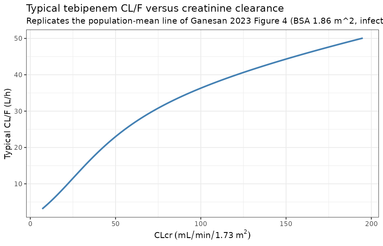
The shape matches the published description: clearance rises approximately linearly up to a creatinine clearance near 80 mL/min/1.73 m^2 and then flattens as the renal arm saturates toward its maximum of 21.1 L/h.
sim_grid |>
  filter(CRCL %in% c(20, 30, 50, 72, 90, 120, 190)) |>
  transmute(
    CRCL,
    `CL_NR (L/h)` = round(cl_nonren, 2),
    `CL_R (L/h)`  = round(cl_renal, 2),
    `CL/F (L/h)`  = round(clf, 2),
    `Renal fraction` = round(cl_renal / clf, 3)
  ) |>
  dplyr::rename(`CLcr (mL/min/1.73 m2)` = CRCL) |>
knitr::kable(caption = "Typical clearance decomposition across the observed creatinine-clearance range.")| CLcr (mL/min/1.73 m2) | CL_NR (L/h) | CL_R (L/h) | CL/F (L/h) | Renal fraction |
|---|---|---|---|---|
| 20 | 5.77 | 3.22 | 8.99 | 0.358 |
| 30 | 7.73 | 6.32 | 14.05 | 0.450 |
| 50 | 11.18 | 11.80 | 22.98 | 0.514 |
| 72 | 14.55 | 15.49 | 30.04 | 0.516 |
| 90 | 17.09 | 17.22 | 34.31 | 0.502 |
| 120 | 21.03 | 18.81 | 39.84 | 0.472 |
| 190 | 29.31 | 20.17 | 49.49 | 0.408 |
Which non-renal-clearance intercept is right?
Ganesan 2023 Table 2 reports CL_NR = 15.6 L/h (%SEM
5.87) with sampling-importance-resampling statistics of mean 15.7,
median 15.7, and a 90% confidence interval of [14.4, 17.1]. Printed
Equation 1, however, reads
CL_NR = 10.2 * (CLcr / 79.32)^0.722. Every other constant
in Equations 1-6 reproduces its Table 2 counterpart exactly, so one of
these two numbers is a typographical error. The check below
discriminates between them using the only assumption-light comparison
the paper offers.
ADAPT-PO enrolled 647 patients, of whom 55 (8.5%) had baseline creatinine clearance at or below 50 mL/min/1.73 m^2 and received 300 mg q8h; the remaining 595 received 600 mg q8h. Because the low-renal-function stratum is only 8.5% of the cohort, the median creatinine clearance of the 600 mg stratum must sit very close to the overall ADAPT-PO median of 72.2 mL/min/1.73 m^2. Table 3 reports a median CL/F of 30.7 L/h for that stratum.
mod_eq1 <- rxode2::ini(mod, lcl_nonren = log(10.2))
#> ℹ parameter labels from comments will be replaced by 'label()'
#> Warning: some etas defaulted to non-mu referenced, possible parsing error: etalcl_patient, etaiov_ka_1, etaiov_ka_2
#> as a work-around try putting the mu-referenced expression on a simple line
#> ℹ change initial estimate of `lcl_nonren` to `2.32238772029023`

check_events <- tibble(
  id               = 1:3,
  CRCL             = c(72.2, 74.2, 78.0),
  BSA              = 1.86,
  HT               = 169,
  DIS_HEALTHY      = 0,
  FED              = 0,
  DOSE_TBPPI_MG    = 600,
  STUDY_SPR994_104 = 0,
  OCC              = 1
) |>
  tidyr::crossing(time = c(0, 1)) |>
  mutate(amt = NA_real_, evid = 0L, cmt = "central", dvid = 1L)

clf_at <- function(model, events) {
  rxode2::rxSolve(model, events = events, omega = NA,
                  keep = "CRCL", useLinCmt = FALSE) |>
    as.data.frame() |>
    filter(time == 1) |>
    transmute(CRCL, clf = cl_nonren + cl_renal)
}

bind_rows(
  clf_at(mod,     check_events) |> mutate(variant = "Table 2 (CL_NR = 15.6)"),
  clf_at(mod_eq1, check_events) |> mutate(variant = "Equation 1 (CL_NR = 10.2)")
) |>
  mutate(
    `Published Table 3 median CL/F (L/h)` = 30.7,
    `% difference` = round(100 * (clf - 30.7) / 30.7, 1),
    clf = round(clf, 2)
  ) |>
  tidyr::pivot_wider(names_from = variant, values_from = c(clf, `% difference`)) |>
  dplyr::rename(`CLcr (mL/min/1.73 m2)` = CRCL) |>
  knitr::kable(
    caption = paste(
      "Typical CL/F for an infected patient at BSA 1.86 m^2 near the ADAPT-PO",
      "median creatinine clearance, under the two candidate CL_NR values,",
      "against the Table 3 median for the 600 mg q8h stratum (n = 595)."
    )
  )
#> Warning: multi-subject simulation without without 'omega'
#> Warning: multi-subject simulation without without 'omega'| CLcr (mL/min/1.73 m2) | Published Table 3 median CL/F (L/h) | clf_Table 2 (CL_NR = 15.6) | clf_Equation 1 (CL_NR = 10.2) | % difference_Table 2 (CL_NR = 15.6) | % difference_Equation 1 (CL_NR = 10.2) |
|---|---|---|---|---|---|
| 72.2 | 30.7 | 30.09 | 25.04 | -2.0 | -18.4 |
| 74.2 | 30.7 | 30.62 | 25.47 | -0.3 | -17.0 |
| 78.0 | 30.7 | 31.57 | 26.24 | 2.8 | -14.5 |
Across the plausible range of median creatinine clearance for the 600 mg stratum the Table 2 value reproduces the published median within a couple of percent, while the Equation 1 value is 15-20% low. Combined with the three-way corroboration of 15.6 by the SIR resample statistics, the model file uses 15.6 and treats the 10.2 in Equation 1 as a typographical error. The same comparison cannot be run against the 300 mg stratum because the median creatinine clearance within a 30-50 mL/min/1.73 m^2 band is not reported and is not recoverable from the pooled summary.
Food effect (replicates Figure 1)
Study 101 dosed food-effect cohorts under fasted and fed conditions at 300 mg and 600 mg. Ganesan 2023 Figure 1 shows that food slowed absorption – fasted profiles peak near 0.75-1 h, fed profiles near 2 h – without materially changing exposure.
set.seed(20230615)

n_food <- 60L

make_healthy_cohort <- function(n, dose_mg, fed, id_offset) {
  subj <- tibble(
    id               = id_offset + seq_len(n),
    HT               = pmin(pmax(rnorm(n, 176, 7), 160), 198),
    BSA              = pmin(pmax(rlnorm(n, log(1.90), 0.07), 1.60), 2.30),
    CRCL             = pmin(pmax(rlnorm(n, log(120), 0.15), 80), 165),
    DIS_HEALTHY      = 1,
    FED              = fed,
    DOSE_TBPPI_MG    = dose_mg,
    STUDY_SPR994_104 = 0,
    OCC              = 1,
    arm              = paste0(dose_mg, " mg, ", ifelse(fed == 1, "fed", "fasted"))
  )

  doses <- subj |>
    mutate(time = 0, amt = dose_mg, evid = 1L, cmt = "depot", dvid = NA_integer_)

  obs <- subj |>
    tidyr::crossing(time = c(seq(0, 4, by = 0.25), seq(4.5, 12, by = 0.5))) |>
    mutate(amt = NA_real_, evid = 0L, cmt = "central", dvid = 1L)

  bind_rows(doses, obs) |> arrange(id, time, desc(evid))
}

food_events <- bind_rows(
  make_healthy_cohort(n_food, 300, 0, id_offset =   0L),
  make_healthy_cohort(n_food, 300, 1, id_offset =  60L),
  make_healthy_cohort(n_food, 600, 0, id_offset = 120L),
  make_healthy_cohort(n_food, 600, 1, id_offset = 180L)
)
stopifnot(!anyDuplicated(food_events[, c("id", "time", "evid")]))
sim_food <-
  rxode2::rxSolve(
    mod,
    events    = food_events,
    keep      = c("arm", "DOSE_TBPPI_MG", "FED"),
    useLinCmt = FALSE
  ) |>
  as.data.frame()

food_summary <- sim_food |>
  filter(time > 0) |>
  group_by(arm, DOSE_TBPPI_MG, FED, time) |>
  summarise(
    p25 = quantile(Cc, 0.25),
    p50 = median(Cc),
    p75 = quantile(Cc, 0.75),
    .groups = "drop"
  ) |>
  mutate(
    dose_label = paste0("Tebipenem ", DOSE_TBPPI_MG, " mg single dose"),
    fed_label  = ifelse(FED == 1, "Fed", "Fasted")
  )

ggplot(food_summary, aes(x = time, y = p50 * 1000, colour = fed_label, linetype = fed_label)) +
  geom_ribbon(aes(ymin = p25 * 1000, ymax = p75 * 1000, fill = fed_label),
              alpha = 0.15, colour = NA) +
  geom_line(linewidth = 0.8) +
  facet_wrap(~dose_label) +
  scale_y_log10(limits = c(10, 8000)) +
  coord_cartesian(xlim = c(0, 12)) +
  labs(
    x = "Nominal time (h)",
    y = "Tebipenem plasma concentration (ng/mL)",
    colour = NULL, fill = NULL, linetype = NULL,
    title = "Simulated food effect in healthy subjects",
    subtitle = "Median (25th-75th percentile); replicates Ganesan 2023 Figure 1"
  ) +
  theme_bw() +
  theme(legend.position = "bottom")
#> Warning: Removed 35 rows containing missing values or values outside the scale range
#> (`geom_ribbon()`).
#> Warning: Removed 17 rows containing missing values or values outside the scale range
#> (`geom_line()`).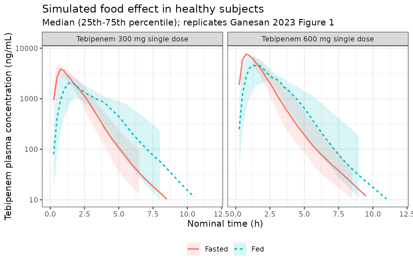
sim_food |>
  filter(time > 0) |>
  group_by(arm, id) |>
  slice_max(Cc, n = 1, with_ties = FALSE) |>
  ungroup() |>
  group_by(arm) |>
  summarise(
    `Median Tmax (h)`     = round(median(time), 2),
    `Median Cmax (ug/mL)` = round(median(Cc), 2),
    .groups = "drop"
  ) |>
  dplyr::rename(Arm = arm) |>
knitr::kable(caption = "Simulated median Tmax and Cmax by dose and prandial state.")| Arm | Median Tmax (h) | Median Cmax (ug/mL) |
|---|---|---|
| 300 mg, fasted | 1.00 | 4.23 |
| 300 mg, fed | 2.00 | 2.43 |
| 600 mg, fasted | 1.00 | 8.21 |
| 600 mg, fed | 1.62 | 5.55 |
The simulated fasted profiles peak near 0.75 h and the fed profiles
near 2 h, matching Figure 1. This is also the independent evidence that
Equation 6 assigns the two Ka values correctly and that Table 2
transposes their row labels: with a mean transit time of
(n_transit + 1) / Ka, the fasted healthy value of
3.04 * 1.368 = 4.16 1/h gives roughly 0.96 h and the fed
healthy value of 1.23 * 1.368 = 1.68 1/h gives roughly 2.4
h. Had the labels in Table 2 been taken at face value, the fed profiles
would have peaked earlier than the fasted ones, contradicting
both Figure 1 and the Results narrative that “the presence of food
slowed the rate of tebipenem absorption”.
ADAPT-PO virtual cohort and PKNCA validation
ADAPT-PO patients received 600 mg q8h, reduced to 300 mg q8h when baseline creatinine clearance was between 30 and 50 mL/min/1.73 m^2. Ganesan 2023 Table 3 reports day-1 AUC0-24 and Cmax by that stratification, derived from individual post-hoc profiles.
Creatinine clearance is drawn from a lognormal calibrated to the ADAPT-PO median of 72.2 mL/min/1.73 m^2 and then truncated into each protocol-defined stratum; height and body surface area are drawn to match the ADAPT-PO medians and ranges of Table 1. The achieved covariate medians are reported alongside the results so the reader can judge how much of any discrepancy is attributable to the reconstruction rather than to the model.
set.seed(20230616)

n_arm <- 150L

make_adapt_cohort <- function(n, dose_mg, crcl_lo, crcl_hi, id_offset) {
  crcl <- rlnorm(200 * n, log(72.2), 0.35)
  crcl <- crcl[crcl > crcl_lo & crcl <= crcl_hi]
  stopifnot(length(crcl) >= n)
  crcl <- crcl[seq_len(n)]

  subj <- tibble(
    id               = id_offset + seq_len(n),
    CRCL             = crcl,
    HT               = pmin(pmax(rnorm(n, 168, 11), 140), 200),
    BSA              = pmin(pmax(rlnorm(n, log(1.86), 0.14), 1.32), 2.70),
    DIS_HEALTHY      = 0,
    FED              = 0,
    DOSE_TBPPI_MG    = dose_mg,
    STUDY_SPR994_104 = 0,
    OCC              = 1,
    regimen          = paste0(dose_mg, " mg q8h")
  )

  doses <- subj |>
    tidyr::crossing(time = c(0, 8, 16)) |>
    mutate(amt = dose_mg, evid = 1L, cmt = "depot", dvid = NA_integer_)

  obs <- subj |>
    tidyr::crossing(time = sort(unique(c(seq(0, 24, by = 0.25))))) |>
    mutate(amt = NA_real_, evid = 0L, cmt = "central", dvid = 1L)

  bind_rows(doses, obs) |> arrange(id, time, desc(evid))
}

adapt_events <- bind_rows(
  make_adapt_cohort(n_arm, 300, 30, 50,  id_offset =   0L),
  make_adapt_cohort(n_arm, 600, 50, 250, id_offset = 150L)
)
adapt_events |>
  distinct(id, regimen, CRCL, HT, BSA) |>
  group_by(regimen) |>
  summarise(
    `Median CLcr (mL/min/1.73 m2)` = round(median(CRCL), 1),
    `CLcr range`                   = paste0(round(min(CRCL), 1), " - ", round(max(CRCL), 1)),
    `Median height (cm)`           = round(median(HT), 1),
    `Median BSA (m2)`              = round(median(BSA), 2),
    n                              = dplyr::n(),
    .groups = "drop"
  ) |>
  dplyr::rename(Regimen = regimen) |>
knitr::kable(caption = "Achieved covariate distributions of the ADAPT-PO virtual cohort.")| Regimen | Median CLcr (mL/min/1.73 m2) | CLcr range | Median height (cm) | Median BSA (m2) | n |
|---|---|---|---|---|---|
| 300 mg q8h | 43.5 | 32.2 - 49.9 | 167.3 | 1.82 | 150 |
| 600 mg q8h | 81.1 | 50.1 - 151.3 | 167.1 | 1.85 | 150 |
sim_adapt <-
  rxode2::rxSolve(
    mod,
    events    = adapt_events,
    keep      = c("regimen", "CRCL", "BSA", "DOSE_TBPPI_MG"),
    useLinCmt = FALSE
  ) |>
  as.data.frame()

ggplot(
  sim_adapt |>
    filter(time > 0) |>
    group_by(regimen, time) |>
    summarise(p05 = quantile(Cc, 0.05), p50 = median(Cc),
              p95 = quantile(Cc, 0.95), .groups = "drop"),
  aes(x = time, y = p50, colour = regimen, fill = regimen)
) +
  geom_ribbon(aes(ymin = p05, ymax = p95), alpha = 0.15, colour = NA) +
  geom_line(linewidth = 0.8) +
  scale_y_log10() +
  labs(
    x = "Time after first dose on day 1 (h)",
    y = "Tebipenem plasma concentration (ug/mL)",
    colour = NULL, fill = NULL,
    title = "Simulated day-1 tebipenem profiles in ADAPT-PO patients",
    subtitle = "Median (5th-95th percentile) by protocol-defined renal-function regimen"
  ) +
  theme_bw() +
  theme(legend.position = "bottom")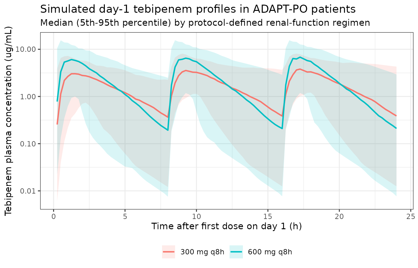
nca_conc <- sim_adapt |>
  filter(!is.na(Cc)) |>
  select(id, time, Cc, regimen)

nca_dose <- adapt_events |>
  filter(evid == 1) |>
  select(id, time, amt, regimen)

conc_obj <- PKNCA::PKNCAconc(
  nca_conc,
  Cc ~ time | regimen + id,
  concu = "ug/mL",
  timeu = "h"
)
dose_obj <- PKNCA::PKNCAdose(
  nca_dose,
  amt ~ time | regimen + id,
  doseu = "mg"
)

intervals <- data.frame(
  start   = 0,
  end     = 24,
  cmax    = TRUE,
  tmax    = TRUE,
  auclast = TRUE
)

nca_res <- PKNCA::pk.nca(PKNCA::PKNCAdata(conc_obj, dose_obj, intervals = intervals))
published <- tibble::tribble(
  ~regimen,      ~cmax, ~auclast,
  "300 mg q8h",  6.68,  59.2,
  "600 mg q8h",  7.98,  60.5
)

cmp <- nlmixr2lib::ncaComparisonTable(
  simulated     = nca_res,
  reference     = published,
  by            = "regimen",
  units         = c(cmax = "ug/mL", auclast = "ug*h/mL"),
  tolerance_pct = 20
)

knitr::kable(
  cmp,
  caption = paste(
    "Simulated day-1 exposure versus Ganesan 2023 Table 3 medians for",
    "ADAPT-PO patients. * differs from the published value by more than 20%."
  ),
  align = c("l", "l", "r", "r", "r")
)| NCA parameter | regimen | Reference | Simulated | % diff |
|---|---|---|---|---|
| Cmax (ug/mL) | 300 mg q8h | 6.68 | 4.68 | -29.9%* |
| Cmax (ug/mL) | 600 mg q8h | 7.98 | 8.33 | +4.4% |
| AUClast (ug*h/mL) | 300 mg q8h | 59.2 | 43.9 | -25.8%* |
| AUClast (ug*h/mL) | 600 mg q8h | 60.5 | 62.3 | +2.9% |
- differs from reference by more than ±20%.
The 600 mg q8h stratum – 595 of the 647 ADAPT-PO patients – reproduces the published medians closely: Cmax within about 4% and day-1 AUC0-24 within about 3%. The 300 mg q8h stratum is flagged: simulated Cmax and AUC0-24 both fall roughly 25-30% below the published medians. The arithmetic is transparent. At the achieved median creatinine clearance of that virtual arm the model predicts a typical CL/F near 20 L/h, whereas Table 3 reports a median post-hoc CL/F of 15.7 L/h for the corresponding patients, and 900 mg of daily dose divided by those two clearances is exactly the observed gap.
Three things plausibly contribute, none of which is a defect in the transcription:
- The stratum’s true median creatinine clearance is not reported. Table 1 gives only the pooled ADAPT-PO median (72.2 mL/min/1.73 m^2), so the median within the 30-50 mL/min/1.73 m^2 band has to be reconstructed. The virtual arm lands at 43.5; the model reproduces the published CL/F of 15.7 L/h at a creatinine clearance near 33 mL/min/1.73 m^2, which is inside the band but toward its floor.
- Body size is not matched within the stratum. Patients with reduced renal function in this population are older and smaller, and CL/F carries a linear body-surface-area slope of 0.479 per m^2. The virtual arm is drawn from the pooled ADAPT-PO body-surface-area distribution rather than a stratum-specific one.
- The published values are medians of shrunken post-hoc estimates from sparse phase 3 sampling in a subgroup of only 55 patients, whereas the simulated values are medians of the model’s own predictions.
The discrepancy is not evidence about the CL_NR
ambiguity discussed earlier: both candidate values over-predict CL/F in
this stratum (about 20 L/h with 15.6 and about 17 L/h with 10.2 at a
creatinine clearance of 43.5), so the 600 mg stratum remains the
discriminating comparison. No parameter was adjusted to close the
gap.
Renal recovery
The renal arm of clearance drives the cumulative urine compartment,
so the fraction of an absorbed dose recovered unchanged in urine is
CL_R / (CL_NR + CL_R) and falls as renal function declines.
The check below reads the urine state out of the same ADAPT-PO
simulation.
sim_adapt |>
  filter(time == 24) |>
  mutate(
    crcl_band = cut(
      CRCL,
      breaks = c(30, 50, 75, 100, 250),
      labels = c("30-50", "50-75", "75-100", ">100"),
      include.lowest = TRUE
    ),
    fe = urine / (3 * DOSE_TBPPI_MG)
  ) |>
  group_by(regimen, crcl_band) |>
  summarise(
    n = dplyr::n(),
    `Median fraction of day-1 dose in urine` = round(median(fe), 3),
    `Predicted renal fraction of CL/F`       = round(median(cl_renal / (cl_renal + cl_nonren)), 3),
    .groups = "drop"
  ) |>
  filter(n > 0) |>
  dplyr::rename(Regimen = regimen, `CLcr band (mL/min/1.73 m2)` = crcl_band) |>
knitr::kable(caption = "Simulated day-1 urinary recovery by renal-function band.")| Regimen | CLcr band (mL/min/1.73 m2) | n | Median fraction of day-1 dose in urine | Predicted renal fraction of CL/F |
|---|---|---|---|---|
| 300 mg q8h | 30-50 | 150 | 0.482 | 0.503 |
| 600 mg q8h | 50-75 | 56 | 0.511 | 0.518 |
| 600 mg q8h | 75-100 | 60 | 0.503 | 0.508 |
| 600 mg q8h | >100 | 34 | 0.468 | 0.474 |
At 24 h the day-1 urinary recovery sits slightly below the renal fraction of clearance because drug remaining in the body at the end of day 1 has not yet been excreted; the gap narrows as renal function – and therefore the elimination rate – increases.
Assumptions and deviations
Errata and internal inconsistencies in the source
CL_NRintercept: Table 2 says 15.6 L/h, Equation 1 says 10.2. Table 2 reports 15.6 with %SEM 5.87 and SIR statistics of mean 15.7, median 15.7, 90% CI [14.4, 17.1]; Equation 1 printsCL_NR = 10.2 * (CLcr / 79.32)^0.722. Every other constant in Equations 1-6 matches its Table 2 counterpart exactly. The model file uses 15.6, because it is the value in the parameter-estimate table, is corroborated three separate ways by the resampling analysis, and is the only one of the two that reproduces the Table 3 median CL/F of the 600 mg q8h stratum (n = 595, 92% of the ADAPT-PO patients) – see the discrimination table above.Table 2’s two Ka rows are transposed. Table 2 lists “Ka (fasted) 1.23” and “Ka (fed) 3.04”. Equation 6 writes
Ka = [3.04 * FAST + 1.23 * (1 - FAST)] * ..., assigning 3.04 to the fasted state; the Results narrative states that “the presence of food slowed the rate of tebipenem absorption”; and Figure 1 shows the fasted profiles peaking roughly an hour earlier than the fed profiles. The model file therefore uses Ka = 3.04 1/h fasted and 1.23 1/h fed, i.e. the equation’s assignment, and treats the Table 2 row labels as transposed.Direction of the infection-status effect on Ka. Equation 6 contains
[1 + 0.368 * (1 - Infected)], which makes absorption 36.8% faster in healthy subjects, whereas the Discussion states that absorption was “faster in infected patients”. Equations 4 and 5 use the same(1 - Infected)construction for Vc/F and Vp/F, so the equation set is internally consistent, and the Tmax values it produces for healthy subjects agree with Figure 1. The equation is implemented as printed. The authors themselves caution that “the impact of infection status on absorption rate should be interpreted with caution as the PK sampling scheme in phase 3 patients was relatively uninformative for the estimation of Ka.”IIV on Vp/F. The Results section describing the simplification of the full multivariable model states that “the IIV term for Vp/F was removed due to excessive shrinkage”, but Table 2 (the final model) reports it as 0.0115 (10.7 %CV, shrinkage 77.3%), and both the Results and the Discussion quote 10.7% for Vp/F as the low end of the final-model IIV range. The term is retained here, following Table 2.
Reference creatinine clearance of 79.32. Equation 1 normalizes to 79.32 mL/min/1.73 m^2, which is not the pooled median reported in Table 1 (74.2) and is presumably the analysis-set mean. It is used as printed.
Modelling choices
Urine residual error. Ganesan 2023 Table 2 reports a combined residual model for urine: proportional 0.298 (54.6 %CV) plus additive 482 (21.9 ng/mL). The additive term is annotated in concentration units, but the Methods describe fitting “urine amounts” and no urine volumes are reported, so the additive component cannot be placed on the cumulative- amount observable that the model exposes. Only the proportional component is carried on
urineAmt; the additive component is documented here and in the model file rather than being converted with an invented urine volume.Fixed cohort anchors for the split CL/F IIV. Ganesan 2023 estimated separate CL/F IIV variances for healthy phase 1 subjects (0.0614) and infected phase 3 patients (0.328) with no accompanying difference in the typical CL/F. Because each random effect must pair with a fixed effect of the same name, the model file introduces
lcl_healthyandlcl_patient, bothfixed(0)(a multiplicative factor of exactly 1), purely to host the two cohort-specific etas. This follows the paired-structural-mean idiom ofKlunder_2017_upadacitinib, and adds no parameter that is not zero by construction.Dose units are pro-drug milligrams. Ganesan 2023 recorded doses as milligrams of TBP-PI, so every apparent parameter is conditioned on the pro-drug-to-tebipenem mass ratio and on the fraction of pro-drug converted (unknown, but expected to be near 100% because pro-drug was not measurable systemically). Simulations must supply
amtin milligrams of TBP-PI-HBr, as done here.
Virtual-cohort assumptions
Covariate distributions are reconstructed, not observed. The original data are not public. Creatinine clearance, height, and body surface area are drawn from parametric distributions matched to the Table 1 medians and ranges of the relevant study, then truncated to the protocol-defined strata. Their achieved medians are reported above.
Prandial state in ADAPT-PO. ADAPT-PO dosed without regard to food and the paper does not report the fed/fasted mix, so the virtual cohort is simulated fasted (
FED = 0). This affects the rate of absorption only, so it moves simulated Cmax but leaves AUC essentially unchanged.Single occasion.
OCC = 1throughout, so only the first interoccasion-variability term on Ka is active. Multi-occasion designs should alternateOCCbetween 1 and 2 across dosing occasions.Race and sex. Neither was retained in the final model, so neither is simulated; both are recorded in
covariatesDataExcludedfor provenance.
Convention check
nlmixr2lib::checkModelConventions("Ganesan_2023_tebipenem")
#> ℹ parameter labels from comments will be replaced by 'label()'
#> Warning: some etas defaulted to non-mu referenced, possible parsing error: etalcl_patient, etaiov_ka_1, etaiov_ka_2
#> as a work-around try putting the mu-referenced expression on a simple line
#>
#> ── Convention check: "Ganesan_2023_tebipenem" ──────────────────────────────────
#> ✔ No convention issues found.