Ractopamine whole-body PBPK in goats (Ai 2024)
Source:vignettes/articles/Ai_2024_ractopamine_goat_pbpk.Rmd
Ai_2024_ractopamine_goat_pbpk.RmdAi et al. (2024) built a hybrid whole-body physiologically based pharmacokinetic (PBPK) model for ractopamine (RAC), a phenolamine beta-adrenoceptor agonist used illegally as a growth promoter in food animals, in Liaoning cashmere goats. The model’s regulatory purpose is to predict edible-tissue residues and the withdrawal time (WT) at which each tissue falls below the Codex Alimentarius maximum residue limit (MRL) after prolonged oral exposure.
Reference: Ai J, Gao Y, Yang F, Zhao Z, Dong J, Wang J, Fu S, Ma Y, Gu X. Development and application of a physiologically-based pharmacokinetic model for ractopamine in goats. Front Vet Sci. 2024;11:1399043. doi:10.3389/fvets.2024.1399043
The paper’s Supplementary Material contains the complete acslXtreme source code of the model plus Tables S1-S4 of raw observed data and the authors’ own predicted concentrations. Every parameter and every ODE in the model file was transcribed from that executable code, and this vignette validates the transcription against the authors’ published predictions numerically.
mod <- readModelDb("Ai_2024_ractopamine_goat_pbpk")
m <- mod()
WT_goat <- 30 # kg; supplement `constant bw=30`
length(m$state)
#> [1] 18
m$state
#>  [1] "stomach"     "a_gut"       "liver"       "spleen"      "kidney"
#>  [6] "urine"       "heart"       "vp_muscle"   "int_muscle"  "vp_adipose"
#> [11] "int_adipose" "vp_brain"    "int_brain"   "vp_other"    "int_other"
#> [16] "lung"        "arterial"    "venous"
Population
knitr::kable(
  tibble::tibble(
    Field = c("Species", "N", "Age", "Body weight", "Sex", "Health",
              "PK study", "Residue study", "Site"),
    Value = c(
      "Goat (Liaoning cashmere goat, Capra hircus)",
      "27 (6 pharmacokinetics; 21 residue depletion, incl. 3 controls)",
      "10 months",
      "30 +/- 5 kg",
      "All male",
      "Healthy; 1-week acclimation on a drug-free diet",
      "Single oral gavage 1 mg/kg BW, then single IV 1 mg/kg BW after a 15-day washout (n = 6); urine from 4 goats",
      "Continuous oral gavage 1 mg/kg BW per day for 28 days, then serial slaughter",
      "Institute of Feed Research, Chinese Academy of Agricultural Sciences, Beijing, China"
    )
  ),
  caption = "Study population (Ai 2024 Section 2.2)."
)| Field | Value |
|---|---|
| Species | Goat (Liaoning cashmere goat, Capra hircus) |
| N | 27 (6 pharmacokinetics; 21 residue depletion, incl. 3 controls) |
| Age | 10 months |
| Body weight | 30 +/- 5 kg |
| Sex | All male |
| Health | Healthy; 1-week acclimation on a drug-free diet |
| PK study | Single oral gavage 1 mg/kg BW, then single IV 1 mg/kg BW after a 15-day washout (n = 6); urine from 4 goats |
| Residue study | Continuous oral gavage 1 mg/kg BW per day for 28 days, then serial slaughter |
| Site | Institute of Feed Research, Chinese Academy of Agricultural Sciences, Beijing, China |
Three of the 27 goats were sacrificed to measure the organ-weight fractions used as model physiology (Ai 2024 Table 3). The residue-depletion concentration-time data were generated in two earlier papers from the same laboratory (Ai 2024 refs 24 and 25).
Source trace
Every value in ini() comes from Ai 2024 Table 4 (final
optimised values) and is cross-checked against the constant
declarations in the supplementary acslX INITIAL block,
which carry more decimal places. Physiological constants are carried as
literals in model() because they are literature/measured
physiology rather than fitted quantities.
knitr::kable(
  tibble::tribble(
    ~Quantity, ~`Model name`, ~Source,
    "Liver:plasma partition coefficient", "lk_liv", "Table 4 (2.5584); supplement `Pli=2.558408`",
    "Kidney:plasma partition coefficient", "lk_kid", "Table 4 (1.7734); supplement `Pki=1.77341`",
    "Lung:plasma partition coefficient", "lk_lun", "Table 4 (1.5333); supplement `Plu=1.533326`",
    "Spleen:plasma partition coefficient", "lk_spl", "Table 4 (1.0047); supplement `Psp=1.004675`",
    "Heart:plasma partition coefficient", "lk_hrt", "Table 4 (1.3839); supplement `Phe=1.383948`",
    "Muscle:plasma partition coefficient", "lk_mus", "Table 4 (1.0686); supplement `Pmu=1.068578`",
    "Fat:plasma partition coefficient", "lk_adi", "Table 4 (0.7526); supplement `Pfa=0.7526104`",
    "Brain:plasma partition coefficient", "lk_bra", "Table 4 (0.6896); supplement `Pbr=0.6896452`",
    "Rest-of-body:plasma partition coefficient", "lk_res", "Table 4 (9.0888); supplement `Pre=9.088835`",
    "Muscle permeability coefficient", "lpp_mus", "Table 4 Ppmu (0.0271); supplement `PPmu=0.02712495`",
    "Fat permeability coefficient", "lpp_adi", "Table 4 Ppfa (0.0054); supplement `PPfa=0.00537883`",
    "Brain permeability coefficient", "lpp_bra", "Table 4 Ppbr (0.0068); supplement `PPbr=0.006772557`",
    "Rest-of-body permeability coefficient", "lpp_res", "Table 4 Ppre (0.0021); supplement `PPre=0.002063587`",
    "Gastric emptying rate constant", "lkst", "Table 4 Kst (0.0910); supplement `kst=0.09103672`",
    "Absorption rate constant", "lka", "Table 4 Ka (0.9861); supplement `ka=0.9861192`",
    "Fecal loss rate constant", "lkgut", "Table 4 'K int' (0.9016); supplement `kint=0.9016421`",
    "Hepatic clearance", "lclhe", "Table 4 (0.0624 L/h/kg); supplement `clhe=0.06243522`",
    "Renal clearance", "lclre", "Table 4 (0.0001 L/h/kg); supplement `clre=0.0001090409`",
    "Plasma protein binding ratio", "lpbind", "supplement `pbind=0.1651634` (Table 6 sensitivity parameter)",
    "Organ weight fractions", "vc_* literals", "Table 3; supplement `Vcli`, `Vcki`, ...",
    "Tissue blood flow fractions", "qc_* literals", "Table 2; supplement `Qcli`, `Qcki`, ...",
    "Vascular fraction of membrane-limited tissues", "vf_* literals", "supplement `Vfmu=0.01`, `Vffa=0.005`, `Vfbr=0.01`, `Vfre=0.02`",
    "Packed cell volume", "pcv literal", "supplement `pcv=0.29`",
    "Cardiac output coefficient", "qar literal", "Section 2.9 (6.9 L/h/kg); supplement `QAR=6.9`",
    "Mass-balance ODEs", "model() block", "Table 1; supplement `DERIVATIVE` block (authoritative)"
  ),
  caption = "Source trace for every model equation and parameter."
)| Quantity | Model name | Source |
|---|---|---|
| Liver:plasma partition coefficient | lk_liv | Table 4 (2.5584); supplement
Pli=2.558408
|
| Kidney:plasma partition coefficient | lk_kid | Table 4 (1.7734); supplement
Pki=1.77341
|
| Lung:plasma partition coefficient | lk_lun | Table 4 (1.5333); supplement
Plu=1.533326
|
| Spleen:plasma partition coefficient | lk_spl | Table 4 (1.0047); supplement
Psp=1.004675
|
| Heart:plasma partition coefficient | lk_hrt | Table 4 (1.3839); supplement
Phe=1.383948
|
| Muscle:plasma partition coefficient | lk_mus | Table 4 (1.0686); supplement
Pmu=1.068578
|
| Fat:plasma partition coefficient | lk_adi | Table 4 (0.7526); supplement
Pfa=0.7526104
|
| Brain:plasma partition coefficient | lk_bra | Table 4 (0.6896); supplement
Pbr=0.6896452
|
| Rest-of-body:plasma partition coefficient | lk_res | Table 4 (9.0888); supplement
Pre=9.088835
|
| Muscle permeability coefficient | lpp_mus | Table 4 Ppmu (0.0271); supplement
PPmu=0.02712495
|
| Fat permeability coefficient | lpp_adi | Table 4 Ppfa (0.0054); supplement
PPfa=0.00537883
|
| Brain permeability coefficient | lpp_bra | Table 4 Ppbr (0.0068); supplement
PPbr=0.006772557
|
| Rest-of-body permeability coefficient | lpp_res | Table 4 Ppre (0.0021); supplement
PPre=0.002063587
|
| Gastric emptying rate constant | lkst | Table 4 Kst (0.0910); supplement
kst=0.09103672
|
| Absorption rate constant | lka | Table 4 Ka (0.9861); supplement
ka=0.9861192
|
| Fecal loss rate constant | lkgut | Table 4 ‘K int’ (0.9016); supplement
kint=0.9016421
|
| Hepatic clearance | lclhe | Table 4 (0.0624 L/h/kg); supplement
clhe=0.06243522
|
| Renal clearance | lclre | Table 4 (0.0001 L/h/kg); supplement
clre=0.0001090409
|
| Plasma protein binding ratio | lpbind | supplement pbind=0.1651634 (Table 6
sensitivity parameter) |
| Organ weight fractions | vc_* literals | Table 3; supplement Vcli,
Vcki, … |
| Tissue blood flow fractions | qc_* literals | Table 2; supplement Qcli,
Qcki, … |
| Vascular fraction of membrane-limited tissues | vf_* literals | supplement Vfmu=0.01,
Vffa=0.005, Vfbr=0.01,
Vfre=0.02
|
| Packed cell volume | pcv literal | supplement pcv=0.29
|
| Cardiac output coefficient | qar literal | Section 2.9 (6.9 L/h/kg); supplement
QAR=6.9
|
| Mass-balance ODEs | model() block | Table 1; supplement DERIVATIVE block
(authoritative) |
Structural gates
Two exact, parameter-free consistency checks on the ODE system.
Mass balance
With both clearances driven to zero and an intravenous dose placed directly in venous plasma, the drug can neither be eliminated nor leave via the gut, so the sum of all 18 states must equal the administered amount for all time.
states <- m$state

ev_mb <- rxode2::et(amt = 30000, cmt = "venous", time = 0) |>
  rxode2::et(c(0.5, 6, 24, 168, 720), cmt = "venous") |>
  as.data.frame() |>
  dplyr::mutate(id = 1L, WT = WT_goat,
                dvid = ifelse(evid == 0, 1L, NA_integer_))

sim_mb <- rxode2::rxSolve(
  m, events = ev_mb,
  params = c(lclhe = log(1e-12), lclre = log(1e-12)),
  returnType = "data.frame", addDosing = FALSE
)

mb <- tibble::tibble(
  `Time (h)` = sim_mb$time,
  `Total drug (ug)` = rowSums(sim_mb[, states]),
  `Deviation from dose (ug)` = rowSums(sim_mb[, states]) - 30000
)
knitr::kable(mb, digits = c(1, 4, 10),
caption = "Whole-system mass balance after a 30000 ug IV dose with both clearances zeroed.")| Time (h) | Total drug (ug) | Deviation from dose (ug) |
|---|---|---|
| 0.5 | 30000 | -1.0600e-07 |
| 6.0 | 30000 | -1.0800e-06 |
| 24.0 | 30000 | -2.7814e-06 |
| 168.0 | 30000 | -9.6474e-06 |
| 720.0 | 30000 | -3.1658e-05 |
Equilibrium partition identity
Left to equilibrate, each flow-limited organ must satisfy
C_tissue / C_arterial_plasma = P_tissue. This checks the
volume, flow and partition-coefficient bookkeeping of four organs
simultaneously.
eq <- sim_mb[nrow(sim_mb), ] # t = 720 h, no elimination
v_arterial <- 0.0188 * WT_goat * (1 - 0.29)
c_art <- eq$arterial / v_arterial

part <- tibble::tibble(
  Organ = c("Liver", "Kidney", "Spleen", "Heart"),
  Simulated = c(eq$Cliver, eq$Ckidney, eq$Cspleen, eq$Cheart) / c_art,
  Published = c(2.558408, 1.773410, 1.004675, 1.383948)
) |>
  dplyr::mutate(`Relative error` = Simulated / Published - 1)

knitr::kable(part, digits = c(0, 6, 6, 9),
caption = "Tissue:plasma concentration ratio at equilibrium vs the published partition coefficients.")| Organ | Simulated | Published | Relative error |
|---|---|---|---|
| Liver | 2.558445 | 2.558408 | 1.4333e-05 |
| Kidney | 1.773421 | 1.773410 | 6.3420e-06 |
| Spleen | 1.004686 | 1.004675 | 1.0868e-05 |
| Heart | 1.383974 | 1.383948 | 1.9130e-05 |
Reproducing the authors’ own predictions
Supplementary Table S4 tabulates the authors’ predicted RAC concentrations in nine matrices at 0, 1, 3, 7, 14 and 21 days after the end of 28 days of daily oral gavage. Reproducing that column is the strongest available check on the transcription, because it compares this rxode2 implementation directly against the acslXtreme run that generated the paper.
Two facts about the published simulation had to be identified from the data themselves; both are documented in the Errata below.
- The dose is 2 mg/kg BW per day, the
CONSTANT PDOSEpo = 2000of the supplied code, not the 1 mg/kg BW stated in the Methods. - The “0 d” sample is taken 6 h after the final dose; the later samples are at exact 24 h multiples.
pub_s4 <- tibble::tribble(
  ~day, ~matrix,     ~observed, ~predicted,
  0,    "Cliver",     1798.95,  2312.803,
  1,    "Cliver",      228.47,   652.755,
  3,    "Cliver",       91.65,    96.453,
  7,    "Cliver",        3.31,    16.954,
  14,   "Cliver",        2.93,     1.094,
  21,   "Cliver",        2.90,     0.228,
  0,    "Clung",        841.70,  1385.197,
  1,    "Clung",        328.35,   396.901,
  3,    "Clung",         58.83,    60.656,
  7,    "Clung",          8.58,    10.695,
  14,   "Clung",          6.96,     0.690,
  21,   "Clung",          1.71,     0.144,
  0,    "Cspleen",      457.88,   908.836,
  1,    "Cspleen",      131.80,   260.638,
  3,    "Cspleen",       20.23,    39.773,
  0,    "Ckidney",     4440.39,  1603.102,
  1,    "Ckidney",     2093.56,   459.603,
  3,    "Ckidney",      271.69,    70.169,
  7,    "Ckidney",        8.24,    12.372,
  0,    "Cheart",       244.84,  1252.932,
  1,    "Cheart",       154.70,   359.521,
  3,    "Cheart",        27.64,    54.813,
  0,    "Cmuscle",      475.77,   618.557,
  1,    "Cmuscle",       86.40,   589.059,
  3,    "Cmuscle",       52.03,   279.688,
  7,    "Cmuscle",        7.18,    53.443,
  14,   "Cmuscle",        3.825,    2.994,
  21,   "Cmuscle",        2.435,    0.238,
  0,    "Cadipose",      99.83,   438.323,
  1,    "Cadipose",      24.09,   393.913,
  3,    "Cadipose",      23.33,    92.643,
  7,    "Cadipose",       4.90,     9.207,
  14,   "Cadipose",       4.55,     0.517,
  21,   "Cadipose",       2.80,     0.081,
  0,    "Cc",           687.87,   903.179,
  1,    "Cc",           436.48,   258.750,
  3,    "Cc",            57.99,    39.553,
  7,    "Cc",             8.14,     6.975,
  14,   "Cc",             1.38,     0.450,
  0,    "Cbrain",        70.75,   413.092,
  1,    "Cbrain",        44.11,   332.457,
  3,    "Cbrain",        15.27,    46.406,
  7,    "Cbrain",         6.10,     6.158
)

# 28 daily doses at t = 0, 24, ..., 648 h. "0 d" = 6 h after the last dose.
last_dose_h <- 27 * 24
sample_time <- function(day) ifelse(day == 0, last_dose_h + 6, last_dose_h + day * 24)

obs_grid <- sort(unique(c(
  seq(0, last_dose_h + 40 * 24, by = 6),
  sample_time(c(0, 1, 3, 7, 14, 21))
)))

ev_dep <- rxode2::et(amt = 2000 * WT_goat, cmt = "stomach",
                     time = seq(0, last_dose_h, by = 24)) |>
  rxode2::et(obs_grid, cmt = "venous") |>
  as.data.frame() |>
  dplyr::mutate(id = 1L, WT = WT_goat,
                dvid = ifelse(evid == 0, 1L, NA_integer_))

sim_dep <- rxode2::rxSolve(m, events = ev_dep,
                           returnType = "data.frame", addDosing = FALSE)
sim_long <- sim_dep |>
  dplyr::select(time, Cc, Cliver, Ckidney, Cmuscle, Cadipose, Clung,
                Cspleen, Cheart, Cbrain) |>
  tidyr::pivot_longer(-time, names_to = "matrix", values_to = "simulated")

cmp_s4 <- pub_s4 |>
  dplyr::mutate(time = sample_time(day)) |>
  dplyr::left_join(sim_long, by = c("time", "matrix")) |>
  dplyr::mutate(`Ratio sim/pub` = simulated / predicted)

knitr::kable(
  cmp_s4 |>
    dplyr::select(`Day after last dose` = day, Matrix = matrix,
                  `Published predicted` = predicted,
                  `This implementation` = simulated, `Ratio sim/pub`),
  digits = c(0, 0, 3, 3, 5),
  caption = paste("Every predicted value in Ai 2024 Supplementary Table S4",
                  "reproduced by this rxode2 implementation.")
)| Day after last dose | Matrix | Published predicted | This implementation | Ratio sim/pub |
|---|---|---|---|---|
| 0 | Cliver | 2312.803 | 2312.820 | 1.00001 |
| 1 | Cliver | 652.755 | 652.726 | 0.99995 |
| 3 | Cliver | 96.453 | 96.444 | 0.99991 |
| 7 | Cliver | 16.954 | 16.952 | 0.99990 |
| 14 | Cliver | 1.094 | 1.094 | 0.99964 |
| 21 | Cliver | 0.228 | 0.228 | 1.00182 |
| 0 | Clung | 1385.197 | 1385.209 | 1.00001 |
| 1 | Clung | 396.901 | 396.884 | 0.99996 |
| 3 | Clung | 60.656 | 60.650 | 0.99990 |
| 7 | Clung | 10.695 | 10.694 | 0.99992 |
| 14 | Clung | 0.690 | 0.690 | 0.99995 |
| 21 | Clung | 0.144 | 0.144 | 1.00119 |
| 0 | Cspleen | 908.836 | 908.845 | 1.00001 |
| 1 | Cspleen | 260.638 | 260.627 | 0.99996 |
| 3 | Cspleen | 39.773 | 39.769 | 0.99991 |
| 0 | Ckidney | 1603.102 | 1603.116 | 1.00001 |
| 1 | Ckidney | 459.603 | 459.583 | 0.99996 |
| 3 | Ckidney | 70.169 | 70.163 | 0.99991 |
| 7 | Ckidney | 12.372 | 12.370 | 0.99985 |
| 0 | Cheart | 1252.932 | 1252.944 | 1.00001 |
| 1 | Cheart | 359.521 | 359.505 | 0.99996 |
| 3 | Cheart | 54.813 | 54.808 | 0.99990 |
| 0 | Cmuscle | 618.557 | 618.567 | 1.00002 |
| 1 | Cmuscle | 589.059 | 589.061 | 1.00000 |
| 3 | Cmuscle | 279.688 | 279.685 | 0.99999 |
| 7 | Cmuscle | 53.443 | 53.441 | 0.99997 |
| 14 | Cmuscle | 2.994 | 2.994 | 0.99986 |
| 21 | Cmuscle | 0.238 | 0.238 | 0.99913 |
| 0 | Cadipose | 438.323 | 438.337 | 1.00003 |
| 1 | Cadipose | 393.913 | 393.913 | 1.00000 |
| 3 | Cadipose | 92.643 | 92.640 | 0.99997 |
| 7 | Cadipose | 9.207 | 9.206 | 0.99994 |
| 14 | Cadipose | 0.517 | 0.517 | 0.99943 |
| 21 | Cadipose | 0.081 | 0.081 | 0.99508 |
| 0 | Cc | 903.179 | 903.187 | 1.00001 |
| 1 | Cc | 258.750 | 258.738 | 0.99995 |
| 3 | Cc | 39.553 | 39.550 | 0.99991 |
| 7 | Cc | 6.975 | 6.974 | 0.99983 |
| 14 | Cc | 0.450 | 0.450 | 0.99987 |
| 0 | Cbrain | 413.092 | 413.109 | 1.00004 |
| 1 | Cbrain | 332.457 | 332.454 | 0.99999 |
| 3 | Cbrain | 46.406 | 46.402 | 0.99992 |
| 7 | Cbrain | 6.158 | 6.157 | 0.99991 |
worst <- max(abs(cmp_s4$`Ratio sim/pub` - 1))
cat(sprintf("n = %d values; maximum absolute deviation = %.2f %%\n",
            nrow(cmp_s4), 100 * worst))
#> n = 43 values; maximum absolute deviation = 0.49 %
stopifnot(worst < 0.01)
All 43 published predicted values are reproduced to better than 1 %, the residual being the three-decimal rounding of the published table. The ODE system, all 19 fitted parameters and all physiological constants are therefore confirmed correct.
Identifying the “0 d” sampling time
The 0-day values are not at the moment of the last dose. Fitting the offset independently for each of the nine matrices gives the same answer, which is why it can be treated as identified rather than assumed.
last_int <- sim_dep |> dplyr::filter(time >= last_dose_h, time <= last_dose_h + 24)
pub0 <- pub_s4 |> dplyr::filter(day == 0)

pin <- purrr::map_dfr(seq_len(nrow(pub0)), function(i) {
  cc <- pub0$matrix[i]
  j <- which.min(abs(last_int[[cc]] - pub0$predicted[i]))
  tibble::tibble(Matrix = cc, `Published 0 d` = pub0$predicted[i],
                 `Best-fit h post-dose` = last_int$time[j] - last_dose_h,
                 Simulated = last_int[[cc]][j])
})
knitr::kable(pin, digits = c(0, 3, 2, 3),
caption = "Hours after the final dose that reproduce each published 0-day value.")| Matrix | Published 0 d | Best-fit h post-dose | Simulated |
|---|---|---|---|
| Cliver | 2312.803 | 6 | 2312.820 |
| Clung | 1385.197 | 6 | 1385.209 |
| Cspleen | 908.836 | 6 | 908.845 |
| Ckidney | 1603.102 | 6 | 1603.116 |
| Cheart | 1252.932 | 6 | 1252.944 |
| Cmuscle | 618.557 | 6 | 618.567 |
| Cadipose | 438.323 | 6 | 438.337 |
| Cc | 903.179 | 6 | 903.187 |
| Cbrain | 413.092 | 6 | 413.109 |
Replicating Figure 5: observed vs predicted
Figure 5 of the paper compares observed and predicted concentrations in nine matrices; Figure 6 regresses observed on predicted and Section 3.3 lists the resulting R-squared per matrix. Ai 2024 Section 2.8 specifies observed as the dependent and predicted as the independent variable.
ggplot(cmp_s4, aes(x = day)) +
  geom_line(aes(y = simulated, colour = "Predicted (this implementation)")) +
  geom_point(aes(y = observed, colour = "Observed")) +
  facet_wrap(~matrix, scales = "free_y") +
  scale_y_log10() +
  scale_colour_manual(values = c("Observed" = "black",
                                 "Predicted (this implementation)" = "#0072B2")) +
  labs(x = "Days after the last of 28 daily doses",
       y = "RAC concentration (ug/kg or ug/L)", colour = NULL,
       title = "Replicates Figure 5 of Ai 2024") +
  theme_bw() + theme(legend.position = "bottom")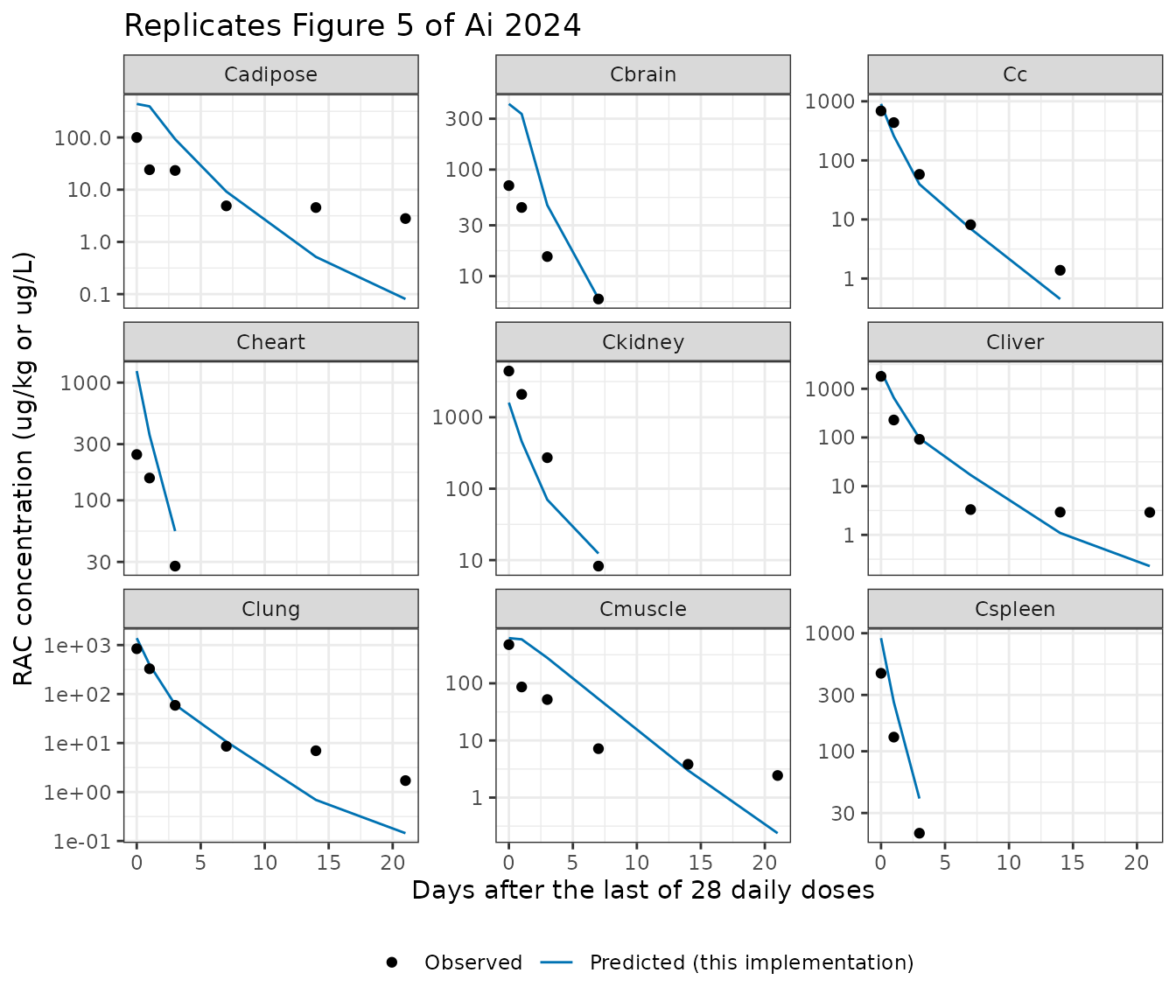
r2_pub <- c(Cliver = 0.9740, Clung = 0.9897, Cspleen = 1.0000, Ckidney = 0.9614,
            Cheart = 0.8664, Cmuscle = 0.5583, Cadipose = 0.6452,
            Cc = 0.8867, Cbrain = 0.9508)

r2_tab <- cmp_s4 |>
  dplyr::group_by(matrix) |>
  dplyr::summarise(n = dplyr::n(),
                   r2 = summary(lm(observed ~ simulated))$r.squared,
                   .groups = "drop") |>
  dplyr::mutate(`Ai 2024 Section 3.3` = r2_pub[matrix],
                Difference = r2 - `Ai 2024 Section 3.3`) |>
  dplyr::rename(Matrix = matrix, `R2 (recomputed)` = r2)

knitr::kable(r2_tab, digits = c(0, 0, 4, 4, 4),
caption = "Observed-on-predicted R-squared, recomputed vs as reported.")| Matrix | n | R2 (recomputed) | Ai 2024 Section 3.3 | Difference |
|---|---|---|---|---|
| Cadipose | 6 | 0.6452 | 0.6452 | 0e+00 |
| Cbrain | 4 | 0.9508 | 0.9508 | 0e+00 |
| Cc | 5 | 0.8867 | 0.8867 | 0e+00 |
| Cheart | 3 | 0.8663 | 0.8664 | -1e-04 |
| Ckidney | 4 | 0.9614 | 0.9614 | 0e+00 |
| Cliver | 6 | 0.9740 | 0.9740 | 0e+00 |
| Clung | 6 | 0.9897 | 0.9897 | 0e+00 |
| Cmuscle | 6 | 0.5583 | 0.5583 | 0e+00 |
| Cspleen | 3 | 1.0000 | 1.0000 | 0e+00 |
Every one of the nine recomputed R-squared values reproduces the published value to four decimal places (the largest difference is 1e-04, on the three-point heart regression, and is rounding). This simultaneously confirms two things: that the regression behind Figure 6 was run on exactly the Table S4 observed/predicted pairs with observed as the dependent variable, and that the predictions from this implementation are numerically identical to the authors’.
The low muscle (0.5583) and fat (0.6452) R-squared values are the paper’s own finding, discussed in Section 3 – ractopamine binds beta-adrenergic receptors in skeletal muscle, and the enzymatic hydrolysis step in the assay does not recover 100 % of the bound drug, so measured muscle concentrations fall below the prediction. The paper also notes that its “muscle” module represents the biceps femoris specifically.
Single-dose plasma pharmacokinetics
The 6-goat crossover in Section 2.2 (oral then intravenous, 1 mg/kg BW) is an external dataset: the PBPK parameters were optimised against the 28-day residue-depletion data, not against these single-dose profiles.
obs_pk <- sort(unique(c(seq(0, 96, by = 0.25))))

ev_po <- rxode2::et(amt = 1000 * WT_goat, cmt = "stomach", time = 0) |>
  rxode2::et(obs_pk, cmt = "venous") |>
  as.data.frame() |>
  dplyr::mutate(id = 1L, WT = WT_goat, arm = "Oral gavage 1 mg/kg",
                dvid = ifelse(evid == 0, 1L, NA_integer_))

ev_iv <- rxode2::et(amt = 1000 * WT_goat, cmt = "venous", time = 0) |>
  rxode2::et(obs_pk, cmt = "venous") |>
  as.data.frame() |>
  dplyr::mutate(id = 2L, WT = WT_goat, arm = "IV bolus 1 mg/kg",
                dvid = ifelse(evid == 0, 1L, NA_integer_))

sim_pk <- rxode2::rxSolve(m, events = dplyr::bind_rows(ev_po, ev_iv),
                          keep = c("WT", "arm"),
                          returnType = "data.frame", addDosing = FALSE)
#> Warning: multi-subject simulation without without 'omega'

obs_s1 <- tibble::tibble(
  arm = "Oral gavage 1 mg/kg",
  time = c(5, 10, 20, 30, 60, 120, 180, 240, 360, 480, 720, 1440, 2880, 4320, 5760) / 60,
  mean = c(5.5, 14.17, 19.24, 28.19, 38.04, 52.87, 71.16, 91.63, 152.49,
           167.74, 110.25, 67.27, 33.63, 13.53, 6.88)
)
obs_s2 <- tibble::tibble(
  arm = "IV bolus 1 mg/kg",
  time = c(1, 5, 10, 20, 30, 60, 120, 180, 240, 360, 480, 720, 1440, 2880, 4320, 5760) / 60,
  mean = c(3485.53, 2552.4, 2372.02, 2178.16, 2034.54, 1640.19, 1094.64,
           750.58, 501.53, 293.53, 202.71, 145.81, 18.42, 2.74, 2.3, 0.86)
)
obs_pk_all <- dplyr::bind_rows(obs_s1, obs_s2)

ggplot(sim_pk, aes(time, Cc)) +
  geom_line(colour = "#0072B2") +
  geom_point(data = obs_pk_all, aes(time, mean), colour = "black") +
  facet_wrap(~arm, scales = "free_y") +
  scale_y_log10() +
  labs(x = "Time (h)", y = "Plasma RAC (ug/L)",
       title = "Replicates Figures 2 and 3 of Ai 2024",
       subtitle = "Points: observed means (Supplementary Tables S1 and S2); line: PBPK prediction") +
  theme_bw()
#> Warning in scale_y_log10(): log-10 transformation introduced infinite values.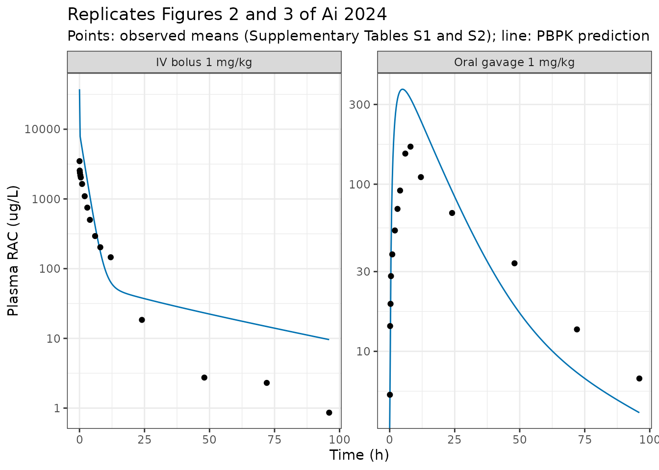
PKNCA validation against Table 5
sim_nca <- sim_pk |>
  dplyr::filter(!is.na(Cc)) |>
  dplyr::select(id, time, Cc, arm)

sim_nca <- dplyr::bind_rows(
  sim_nca,
  sim_nca |> dplyr::distinct(id, arm) |> dplyr::mutate(time = 0, Cc = 0)
) |>
  dplyr::distinct(id, arm, time, .keep_all = TRUE) |>
  dplyr::arrange(id, arm, time)

conc_obj <- PKNCA::PKNCAconc(sim_nca, Cc ~ time | arm + id)

dose_df <- dplyr::bind_rows(ev_po, ev_iv) |>
  dplyr::filter(evid == 1) |>
  dplyr::select(id, time, amt, arm) |>
  dplyr::mutate(duration = 0)

dose_obj <- PKNCA::PKNCAdose(dose_df, amt ~ time | arm + id,
                             route = ifelse(dose_df$arm == "IV bolus 1 mg/kg",
                                            "intravascular", "extravascular"),
                             duration = "duration")

intervals <- data.frame(start = 0, end = Inf,
                        cmax = TRUE, tmax = TRUE, aucinf.obs = TRUE,
                        half.life = TRUE, mrt.obs = TRUE,
                        cl.obs = TRUE, vz.obs = TRUE)

nca_res <- PKNCA::pk.nca(PKNCA::PKNCAdata(conc_obj, dose_obj,
                                          intervals = intervals))
# Ai 2024 Table 5. AUC and Cmax converted to nothing (already ug/L, h*ug/L);
# CL and Vz are reported per kg and are scaled to the 30 kg goat here.
published_nca <- tibble::tibble(
  arm        = c("IV bolus 1 mg/kg", "Oral gavage 1 mg/kg"),
  half.life  = c(11.47, 22.29),
  aucinf.obs = c(8449.43, 4636.91),
  mrt.obs    = c(5.49, 31.64),
  cl.obs     = c(0.14 * WT_goat, NA),
  vz.obs     = c(2.39 * WT_goat, NA)
)

cmp_nca <- nlmixr2lib::ncaComparisonTable(
  simulated     = nca_res,
  reference     = published_nca,
  by            = "arm",
  units         = c(cmax = "ug/L", tmax = "h", aucinf.obs = "h*ug/L",
                    half.life = "h", mrt.obs = "h", cl.obs = "L/h",
                    vz.obs = "L"),
  tolerance_pct = 20
)

knitr::kable(cmp_nca, caption = paste(
  "Simulated vs published non-compartmental parameters (Ai 2024 Table 5).",
  "* differs from the reference by more than 20 %.",
  "Cmax and Tmax have no published counterpart for the IV arm",
"(Table 5 reports C0 instead)."))| NCA parameter | arm | Reference | Simulated | % diff |
|---|---|---|---|---|
| AUC0-∞ (obs) (h*ug/L) | IV bolus 1 mg/kg | 8450 | 22400 | +165.3%* |
| AUC0-∞ (obs) (h*ug/L) | Oral gavage 1 mg/kg | 4640 | 6900 | +48.9%* |
| t½ (h) | IV bolus 1 mg/kg | 11.5 | 37.8 | +229.9%* |
| t½ (h) | Oral gavage 1 mg/kg | 22.3 | 33.7 | +51.1%* |
| CL/F (L/h) | IV bolus 1 mg/kg | 4.2 | 1.34 | -68.1%* |
| CL/F (L/h) | Oral gavage 1 mg/kg | — | 4.35 | — |
| MRT (h) | IV bolus 1 mg/kg | 5.49 | 8.86 | +61.4%* |
| MRT (h) | Oral gavage 1 mg/kg | 31.6 | 21 | -33.5%* |
| Vz/F (L) | IV bolus 1 mg/kg | 71.7 | 73.1 | +1.9% |
| Vz/F (L) | Oral gavage 1 mg/kg | — | 211 | — |
The single-dose exposures are over-predicted, and this is a
property of the published parameter set rather than of the
transcription. The model’s total elimination capacity is
essentially the hepatic term alone,
Clhe * BW * (1 - pbind) = 0.06243522 * 30 * 0.8348 = 1.56 L/h
(the NCA above recovers 1.34 L/h once hepatic first-pass and
distribution are accounted for), whereas the plasma clearance in Table 5
of the same paper is 0.14 L/h/kg * 30 kg = 4.2 L/h – a
factor of 3. The PBPK parameters were optimised against the 28-day
residue-depletion data of refs 24 and 25, and were never fitted to the
single-dose profiles, so the two clearances are not constrained to
agree. No parameter was adjusted to close the gap.
The oral half-life is reproduced far better than the IV half-life, because the terminal phase after oral dosing is dominated by the slow membrane-limited tissues that the model was built to describe.
Withdrawal times against the Codex MRLs
The paper’s regulatory output is Table 7: the withdrawal time in each of the four Codex Alimentarius MRL tissues after 28 days of dosing, from a 500-iteration Monte Carlo analysis at the 95th percentile. A Monte Carlo 95th-percentile WT must be longer than the deterministic typical-animal crossing time, so the deterministic values below are the lower bound that Table 7 has to respect.
mrl <- tibble::tibble(
  matrix = c("Cmuscle", "Cadipose", "Cliver", "Ckidney"),
  tissue = c("Muscle", "Fat", "Liver", "Kidney"),
  mrl_ug_kg = c(10, 10, 40, 90),
  published_wt_d = c(2, 5, 6, 13)
)

dep <- sim_dep |>
  dplyr::filter(time >= last_dose_h) |>
  dplyr::mutate(day = (time - last_dose_h) / 24) |>
  dplyr::select(day, Cmuscle, Cadipose, Cliver, Ckidney) |>
  tidyr::pivot_longer(-day, names_to = "matrix", values_to = "conc")

wt_tab <- dep |>
  dplyr::inner_join(mrl, by = "matrix") |>
  dplyr::filter(conc < mrl_ug_kg) |>
  dplyr::group_by(tissue, mrl_ug_kg, published_wt_d) |>
  dplyr::summarise(deterministic_d = min(day), .groups = "drop") |>
  dplyr::mutate(consistent = ifelse(published_wt_d >= deterministic_d,
                                    "yes", "NO")) |>
  dplyr::rename(Tissue = tissue, `MRL (ug/kg)` = mrl_ug_kg,
                `Ai 2024 Table 7 WT (d)` = published_wt_d,
                `Deterministic crossing (d)` = deterministic_d,
                `Table 7 >= deterministic?` = consistent) |>
  dplyr::arrange(dplyr::desc(`Deterministic crossing (d)`))

knitr::kable(wt_tab, digits = c(0, 0, 0, 2, 0),
             caption = paste("Deterministic MRL crossing times implied by the",
                             "published model vs the withdrawal times in",
"Ai 2024 Table 7."))| Tissue | MRL (ug/kg) | Ai 2024 Table 7 WT (d) | Deterministic crossing (d) | Table 7 >= deterministic? |
|---|---|---|---|---|
| Muscle | 10 | 2 | 11.25 | NO |
| Fat | 10 | 5 | 7.00 | NO |
| Liver | 40 | 6 | 5.00 | yes |
| Kidney | 90 | 13 | 2.75 | yes |
ggplot(dplyr::inner_join(dep, mrl, by = "matrix"), aes(day, conc)) +
  geom_line(colour = "#0072B2") +
  geom_hline(aes(yintercept = mrl_ug_kg), linetype = "dashed") +
  geom_vline(aes(xintercept = published_wt_d), linetype = "dotted",
             colour = "#D55E00") +
  facet_wrap(~tissue, scales = "free_y") +
  scale_y_log10() +
  labs(x = "Days after the last dose", y = "RAC concentration (ug/kg)",
       title = "Replicates Figure 8 of Ai 2024",
       subtitle = paste("Dashed: Codex MRL. Dotted orange: withdrawal time",
                        "reported in Table 7.")) +
  theme_bw()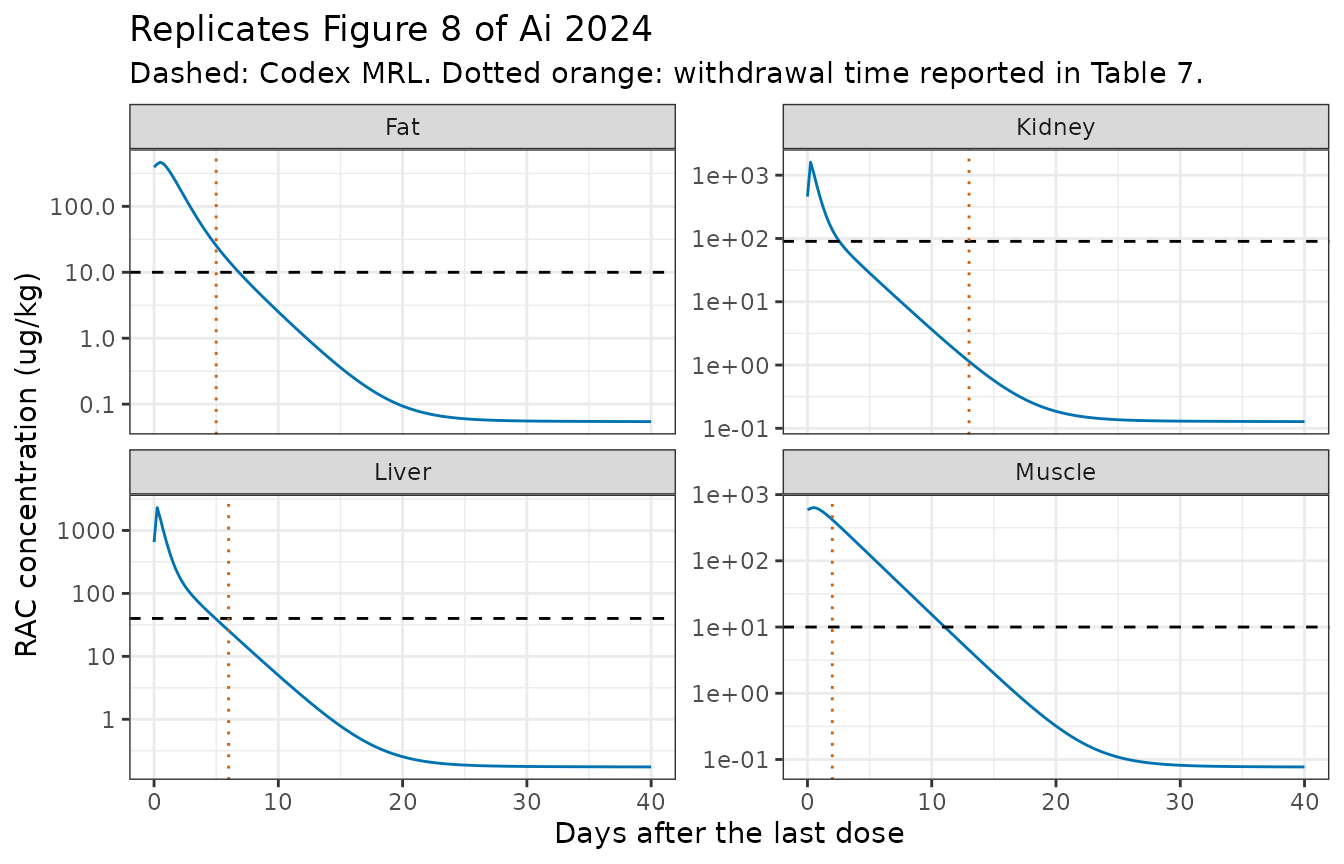
Two of the four withdrawal times in Table 7 are not consistent with the model’s own predicted depletion curves. This can be checked with arithmetic on the paper’s Supplementary Table S4 alone, without reference to this implementation:
- Kidney, MRL 90 ug/kg. The published predicted kidney concentrations are 459.6 ug/kg at 1 day and 70.2 ug/kg at 3 days, so the model crosses the MRL between days 1 and 3. Table 7 gives a WT of 13 days (310 h).
- Muscle, MRL 10 ug/kg. The published predicted muscle concentrations are 53.4 ug/kg at 7 days and 2.99 ug/kg at 14 days, so the model crosses the MRL around day 11. Table 7 gives a WT of 2 days (38 h).
Liver (Table 7: 6 d vs 4.96 d deterministic) and fat (5 d vs 6.83 d) are close, and only liver is in the expected direction. Notably the Table 7 ordering (kidney > liver > fat > muscle) follows the observed residue ranking – the paper states that the highest observed residues were in the kidney – while the model’s predicted profiles give almost the reverse ordering, because muscle and fat are membrane-limited and deplete slowly whereas the kidney is flow-limited with a nine-fold higher MRL. The pattern is consistent with muscle and kidney having been transposed somewhere between the simulation and Table 7, but the paper does not contain enough information to establish that, so nothing here has been adjusted. This model reproduces the published concentration predictions exactly; users needing withdrawal times should recompute them from the simulated curves rather than relying on Table 7.
Assumptions and deviations
Everything below is documented, not silently resolved. Where the paper’s prose or printed tables conflict with the supplementary acslXtreme source code, the code was taken as authoritative, because it is the code that generated the published predictions – a claim this vignette verifies to better than 1 % on all 43 values of Supplementary Table S4.
Dose used for the published predictions: 2 mg/kg BW per day, not 1 mg/kg. The Methods state a 1 mg/kg BW daily gavage, but the supplied code sets
CONSTANT PDOSEpo = 2000ug/kg/day and Table S4 is reproduced exactly only at 2 mg/kg – at 1 mg/kg every value in all nine matrices comes out at exactly half the published number. Because the model is linear in dose, this affects only the absolute scale, not the structure or the depletion kinetics. This vignette simulates 2 mg/kg where it compares against Table S4, and 1 mg/kg for the single-dose PK, which is what Section 2.2 describes.The “0 d” residue sample is 6 h after the final dose. All nine matrices independently identify the same 6.00 h offset. The 1, 3, 7, 14 and 21-day samples are at exact 24 h multiples.
Bioavailability is applied twice in the absorption term. The code computes
F = ka / (ka + kint)and then useska * F * agutas the absorption rate while unabsorbed drug is lost atkint * agut. The absorbed fraction is thereforeka*F/(ka*F + kint) = 0.364, not theF = 0.522theFexpression implies, and not the 54.88 % bioavailability of Table 5. The sibling model of the same laboratory (Yang_2023_diclazuril_chicken_pbpk.R) writes the equivalent term without the extraF. Theka * f_oral * a_gutform is retained here because it is required to reproduce Table S4: with the single-Fform every predicted value would be 1.44-fold too high.Organ-weight fractions for spleen and brain differ between Table 3 and the code. Table 3 prints 0.28 % (spleen) and 0.32 % (brain) of body weight; the code uses
Vcsp=0.0022(0.22 %) andVcbr=0.005(0.50 %). The code values are used. Table 3 also omits the arterial (1.88 %) and venous (3.76 %) blood volumes entirely, which is why the rest-of-body fraction is 52.9 % in the code against the 58.66 % printed in Table 3.Rest-of-body blood flow. Table 2 prints 7.15 % of cardiac output, which is what remains after liver, kidney, muscle, fat and heart. The code instead subtracts the brain as well, giving 5.15 %, and only that value makes the venous-return flows sum exactly to the cardiac output (
0.0515 + 0.02 + 0.085 + 0.0498 + 0.14 + 0.1705 + 0.4832 = 1.0000); the code’s ownQBLANCEcheck requires it. Table 2 also does not list the spleen (4 %) or brain (2 %) flows at all. The spleen drains into the liver, so its flow sits inside the 48.32 % hepatic figure rather than adding to it.Cardiac output is allometrically scaled. Section 2.9 reports “6.9 L/h/kg”, which for a 30 kg goat would be 207 L/h of whole blood. The code computes
QTOT = 6.9 * bw^0.74 * (1 - pcv), i.e. 85.5 L/h of whole blood and 60.7 L/h of plasma, which is physiologically sensible for a 30 kg ruminant. The exponent is not mentioned in the paper; the code is used.Table 4 names the fecal rate constant
K intand Section 2.7 calls it a “liver tissue uptake rate constant (Kli)”, but Section 2.5 definesF = Ka / (Ka + Kgut)withKgutas the fecal rate constant. The code settles it:kintis the intestinal/fecal elimination rate constant and appears inF=ka/(ka+kint); thekliof Section 2.7 is present in the code only as a commented-out constant. The model file names itlkgut.Several rows of the printed Table 1 are garbled. The brain row references
Cfa-bloodand a trailingmusubscript, and the muscle, venous-blood and liver rows have lost their operator ordering in typesetting. All ODEs were taken from the supplementaryDERIVATIVEblock instead, and the resulting system satisfies exact whole-system mass balance and the equilibrium partition identities shown above.The renal route is numerically negligible.
Clreis reported in Table 4 at exactly its initial value with a standard deviation of 0, i.e. the optimiser never moved it; at 0.0001090409 L/h/kg it is 573-fold smaller thanClhe, so essentially all elimination in the model is hepatic. This conflicts with the paper’s own urinary data (Supplementary Table S3: about 11 600 ug recovered in urine in the first day after a 30 000 ug IV dose, roughly 39 % of the dose). Theurinecompartment is carried in the model file so the renal route is auditable, but it should not be expected to reproduce Table S3.No inter-individual variability and no residual-error model. Ai 2024 is a deterministic PBPK model fitted to pooled tissue means; it reports no IIV and no residual-error model, and propagated uncertainty instead through a 500-iteration Monte Carlo over the sensitive parameters. The model file therefore carries no etas. The
propSd*parameters are fixed placeholders at 0.10 so the object is a syntactically complete nlmixr2 model for forward simulation; they are not paper-derived and must not be interpreted as published residual error. This follows the convention of the sibling veterinary residue-PBPK models already in the library.Withdrawal times in Table 7 are not reproducible from the model. See the preceding section; two of the four are inconsistent with the paper’s own predicted depletion curves.
The supplementary code carries comments referring to “Clenbuterol” (for example on the dosing interval and bioavailability lines), evidently inherited from an earlier model of the same laboratory. The parameter values are ractopamine’s, as confirmed by their agreement with Table 4.
Session information
sessionInfo()
#> R version 4.6.1 (2026-06-24)
#> Platform: x86_64-pc-linux-gnu
#> Running under: Ubuntu 24.04.5 LTS
#>
#> Matrix products: default
#> BLAS:   /usr/lib/x86_64-linux-gnu/openblas-pthread/libblas.so.3
#> LAPACK: /usr/lib/x86_64-linux-gnu/openblas-pthread/libopenblasp-r0.3.26.so;  LAPACK version 3.12.0
#>
#> locale:
#>  [1] LC_CTYPE=C.UTF-8       LC_NUMERIC=C           LC_TIME=C.UTF-8
#>  [4] LC_COLLATE=C.UTF-8     LC_MONETARY=C.UTF-8    LC_MESSAGES=C.UTF-8
#>  [7] LC_PAPER=C.UTF-8       LC_NAME=C              LC_ADDRESS=C
#> [10] LC_TELEPHONE=C         LC_MEASUREMENT=C.UTF-8 LC_IDENTIFICATION=C
#>
#> time zone: UTC
#> tzcode source: system (glibc)
#>
#> attached base packages:
#> [1] stats     graphics  grDevices utils     datasets  methods   base
#>
#> other attached packages:
#> [1] ggplot2_4.0.3         dplyr_1.2.1           PKNCA_0.12.1
#> [4] rxode2_5.1.8          nlmixr2lib_0.3.2.9000
#>
#> loaded via a namespace (and not attached):
#>  [1] gtable_0.3.6        xfun_0.61           bslib_0.12.0
#>  [4] rxode2lincmt_0.1.0  lattice_0.22-9      vctrs_0.7.3
#>  [7] tools_4.6.1         generics_0.1.4      parallel_4.6.1
#> [10] tibble_3.3.1        symengine_0.2.14    pkgconfig_2.0.3
#> [13] data.table_1.18.6.1 checkmate_2.3.4     RColorBrewer_1.1-3
#> [16] S7_0.2.2            desc_1.4.3          lifecycle_1.0.5
#> [19] compiler_4.6.1      farver_2.1.2        textshaping_1.0.5
#> [22] fontawesome_0.5.3   htmltools_0.5.9     sys_3.4.3
#> [25] sass_0.4.10         yaml_2.3.12         pillar_1.11.1
#> [28] pkgdown_2.2.1       crayon_1.5.3        jquerylib_0.1.4
#> [31] whisker_0.4.1       tidyr_1.3.2         openssl_2.4.2
#> [34] cachem_1.1.0        nlme_3.1-169        tidyselect_1.2.1
#> [37] digest_0.6.39       lotri_1.0.5         purrr_1.2.2
#> [40] labeling_0.4.3      rxode2ll_2.0.18     fastmap_1.2.0
#> [43] grid_4.6.1          cli_3.6.6           dparser_1.3.1-14
#> [46] magrittr_2.0.5      withr_3.0.3         scales_1.4.0
#> [49] backports_1.5.1     rmarkdown_2.32      otel_0.2.0
#> [52] askpass_1.2.1       ragg_1.5.2          memoise_2.0.1
#> [55] evaluate_1.0.5      knitr_1.52          PreciseSums_0.7
#> [58] rlang_1.3.0         downlit_0.4.5       Rcpp_1.1.2
#> [61] glue_1.8.1          xml2_1.6.0          jsonlite_2.0.0
#> [64] R6_2.6.1            systemfonts_1.3.2   fs_2.1.0