Tenofovir prodrugs in pregnancy (Yu 2026)
Source:vignettes/articles/Yu_2026_tenofovir.Rmd
Yu_2026_tenofovir.RmdModels and source
This paper contributes three model files to
nlmixr2lib, matching the three NONMEM fits the authors
built:
modSemi <- rxode2::rxode2(readModelDb("Yu_2026_tenofovir"))
#> ℹ parameter labels from comments will be replaced by 'label()'
modTfv  <- rxode2::rxode2(readModelDb("Yu_2026_tenofovir_pregnancy_tfv"))
#> ℹ parameter labels from comments will be replaced by 'label()'
modTaf  <- rxode2::rxode2(readModelDb("Yu_2026_tenofovir_pregnancy_taf"))
#> ℹ parameter labels from comments will be replaced by 'label()'- Citation: Yu Y, Brooks KM, Doncel GF, Best BM, Marzinke MA, Mirochnick M, Anderson P, Myer L, Celum C, Heffron R, Coleman J, Joseph Davey D, Hendrix CW, Momper JD, Bies R, Scott RK. Development of a Semi-Mechanistic Population Pharmacokinetic Model for Predicting Tenofovir Disoproxil Fumarate and Tenofovir Alafenamide Exposure in Plasma and Cellular Matrices During Pregnancy and Postpartum. Clin Pharmacokinet. 2026;65(1):133-148. doi:10.1007/s40262-025-01589-y. Structural parameters from Table 2; ordinary differential equations from Results section 3.2.1; pregnancy effects from Results section 3.2.2.
- Article: https://doi.org/10.1007/s40262-025-01589-y
- Supplement (ESM Tables S1 and S2): https://doi.org/10.1007/s40262-025-01589-y (Electronic
Supplementary Material,
40262_2025_1589_MOESM1_ESM.docx)
| Model file | Source | What it is |
|---|---|---|
Yu_2026_tenofovir |
Table 2, Results 3.2.1, Results 3.2.2 | The headline eight-compartment semi-mechanistic model: plasma TAF, plasma TFV after either prodrug, and intracellular TFV-dp in PBMCs and in red cells (DBS), with the pregnancy effects folded in for the clinical trial simulation. |
Yu_2026_tenofovir_pregnancy_tfv |
ESM Table S1, Fig. 4A | The standalone covariate-identification fit for plasma TFV after
TDF: two-compartment, with CL/F estimated separately in
each pregnancy state. |
Yu_2026_tenofovir_pregnancy_taf |
ESM Table S2, Fig. 4B | The standalone covariate-identification fit for plasma TAF:
one-compartment, with relative bioavailability F estimated
separately in each pregnancy state. |
Description of the semi-mechanistic model:
Eight-compartment semi-mechanistic population PK model describing every clinically relevant tenofovir moiety after either prodrug with a single unified parameter set: plasma tenofovir alafenamide (TAF), plasma tenofovir (TFV) arising from both TAF and tenofovir disoproxil fumarate (TDF), and the intracellular active anabolite tenofovir diphosphate (TFV-dp) in peripheral blood mononuclear cells (PBMCs) and in red cells sampled as dried blood spots (DBS). Plasma TAF is one-compartment; plasma TFV is two-compartment with a central and peripheral volume shared between the two prodrug routes. A fraction fm of the TAF eliminated from plasma converts to plasma TFV, of which a fraction frac converts immediately and the remainder passes through a transit compartment at rate ktr, producing the longer TFV half-life seen after TAF. Both intracellular pools are biophase compartments carried directly as concentrations: PBMC TFV-dp is fed by plasma TAF (the dominant route, via cathepsin A) and by plasma TFV, while red-cell TFV-dp is fed by plasma TFV alone because cathepsin A is absent from red cells. TDF is not carried as a state: its plasma half-life is about 24 seconds, so a 300 mg TDF dose is given directly into the tenofovir depot as its 136 mg TFV-equivalent. Pregnancy enters as second-trimester, third-trimester and postpartum fractional shifts on plasma TFV apparent clearance and on relative TAF bioavailability, carried over from the two companion pregnancy sub-models Yu_2026_tenofovir_pregnancy_tfv and Yu_2026_tenofovir_pregnancy_taf. Doses and amount states are in umol; all concentrations, including the two concentration-valued intracellular states, are in umol/L.
Population
Yu 2026 is a secondary analysis pooling four trials in women (Table 1). The structural, non-pregnant model was fitted to healthy HIV-negative volunteers in CONRAD 137 (TDF 300 mg, TAF 10 mg and TAF 25 mg arms; 24 single-dose and 73 multiple-dose participants, who may overlap) and in the directly-observed-therapy DOT-DBS study (TDF 300 mg, 28 participants). CONRAD 137 supplied plasma TFV, plasma TAF and PBMC TFV-dp; DOT-DBS additionally supplied the only DBS TFV-dp data in the analysis.
The pregnancy effects were identified in pregnant and postpartum women with HIV: IMPAACT P1026s (46 participants in the TDF arm and 25 in the TAF arm) and IMPAACT 2026 (28 in the TAF arm). Participants co-administered TAF with a pharmacokinetic booster (cobicistat or ritonavir) were excluded, because P-glycoprotein inhibition raises TAF and TFV concentrations (Methods 2.1). Each pregnant participant was sampled in the second trimester, the third trimester and 6-12 weeks postpartum.
The cohort is entirely female by design. Yu 2026 reports no age, weight or race distributions – populations were deliberately not matched on age or race because covariate data were limited in the pooled datasets and neither factor had previously been identified as a significant covariate on TDF or TAF disposition (Methods 2.1). Plasma TAF was heavily censored (49.9-69.7% of samples below the limit of quantification), handled by the Beal M3 method; PBMC TFV-dp used the M1 method because each sample carried its own limit of quantification.
The same information is available programmatically from the model metadata:
str(readModelDb("Yu_2026_tenofovir")()$population, max.level = 1)
#> List of 9
#>  $ species       : chr "human"
#>  $ n_subjects    : int 224
#>  $ n_studies     : int 4
#>  $ sex_female_pct: num 100
#>  $ disease_state : chr "Women receiving TDF 300 mg or TAF 10-25 mg once daily. The structural (non-pregnant) model was fitted to health"| __truncated__
#>  $ dose_range    : chr "TDF 300 mg once daily (modelled as 136 mg = 474 umol tenofovir) or TAF 25 mg once daily (52.5 umol); the CONRAD"| __truncated__
#>  $ regions       : chr "USA and international IMPAACT network sites; CONRAD 137 and DOT-DBS conducted in the USA"
#>  $ co_medication : chr "Participants co-administered TAF with a pharmacokinetic booster (cobicistat or ritonavir) were excluded, becaus"| __truncated__
#>  $ notes         : chr "n_subjects is the sum of the per-arm participant counts in Table 1 (24 + 73 + 28 + 46 + 25 + 28 = 224); the CON"| __truncated__
Model structure
Yu 2026 Results 3.2.1 prints the eight ordinary differential
equations. Written with this package’s canonical compartment names,
X1..X6 become depot, central,
transit1, depot_tfv, central_tfv,
peripheral1_tfv, and the two biophase states
CPBMC / CDBS become pbmc_tfvdp /
rbc_tfvdp:
| Paper state | Model compartment | Contents |
|---|---|---|
X1 |
depot |
Oral tenofovir alafenamide (TAF) dose |
X2 |
central |
Plasma TAF (amount, umol) |
X3 |
transit1 |
TAF-derived tenofovir en route to plasma (the slow conversion arm) |
X4 |
depot_tfv |
Oral TDF dose, entered as its tenofovir equivalent |
X5 |
central_tfv |
Plasma tenofovir (TFV) |
X6 |
peripheral1_tfv |
Peripheral tenofovir |
CPBMC |
pbmc_tfvdp |
PBMC tenofovir diphosphate (concentration, umol/L) |
CDBS |
rbc_tfvdp |
Red-cell / DBS tenofovir diphosphate (concentration, umol/L) |
Three structural points are worth stating explicitly because they are easy to get wrong:
-
TDF is never a state. Its plasma half-life is about
24 seconds, so Yu 2026 gives “an equivalent 136-mg dose of TFV …
directly when taking 300 mg of TDF” (Methods 2.4.2).
depot_tfvtherefore receives 473.5 umol (136 mg / 287.21 g/mol), not the 300 mg TDF dose. -
The two intracellular pools are concentrations, not
amounts. The paper writes them as
dC/dt, so their influx and efflux constants are plain 1/h rate constants and no volume divides them at the observation step. -
PBMCs are loaded from two different plasma species; red
cells from one. Cathepsin A converts TAF to TFV-dp inside
PBMCs, so
pbmc_tfvdpis fed by both plasma TAF (kinf_pbmc, the dominant route) and plasma TFV (kinf_pbmc_tfv). Cathepsin A is absent from red cells, sorbc_tfvdpis fed by plasma TFV alone (kinf_rbc).
cat(paste(vapply(modSemi$lstExpr, deparse1, character(1)), collapse = "\n"))
TRI2 <- ifelse(TPP > 0, 0, ifelse(EGA >= 14 & EGA < 28, 1, 0))
TRI3 <- ifelse(TPP > 0, 0, ifelse(EGA >= 28, 1, 0))
PP <- ifelse(TPP > 0, 1, 0)
ka <- exp(lka + etalka)
cl <- exp(lcl + etalcl)
vc <- exp(lvc + etalvc)
fm <- exp(lfm)
frac <- exp(lfrac + etalfrac)
ktr <- exp(lktr)
ka_tfv <- exp(lka_tfv + etalka_tfv)
cl_tfv <- exp(lcl_tfv + etalcl_tfv) * (1 + e_tri2_cl_tfv * TRI2 + e_tri3_cl_tfv * TRI3 + e_pp_cl_tfv * PP)
vc_tfv <- exp(lvc_tfv + etalvc_tfv)
vp_tfv <- exp(lvp_tfv)
q_tfv <- exp(lq_tfv)
kinf_pbmc <- exp(lkinf_pbmc + etalkinf_pbmc)
kinf_pbmc_tfv <- exp(lkinf_pbmc_tfv + etalkinf_pbmc_tfv)
keff_pbmc <- exp(lkeff_pbmc + etalkeff_pbmc)
kinf_rbc <- exp(lkinf_rbc)
keff_rbc <- exp(lkeff_rbc)
kel <- cl/vc
kel_tfv <- cl_tfv/vc_tfv
k12_tfv <- q_tfv/vc_tfv
k21_tfv <- q_tfv/vp_tfv
d/dt(depot) <- -ka * depot
d/dt(central) <- ka * depot - kel * central
d/dt(transit1) <- fm * (1 - frac) * kel * central - ktr * transit1
d/dt(depot_tfv) <- -ka_tfv * depot_tfv
d/dt(central_tfv) <- ka_tfv * depot_tfv + fm * frac * kel * central + ktr * transit1 - kel_tfv * central_tfv - k12_tfv * central_tfv + k21_tfv * peripheral1_tfv
d/dt(peripheral1_tfv) <- k12_tfv * central_tfv - k21_tfv * peripheral1_tfv
d/dt(pbmc_tfvdp) <- kinf_pbmc_tfv * (central_tfv/vc_tfv) + kinf_pbmc * (central/vc) - keff_pbmc * pbmc_tfvdp
d/dt(rbc_tfvdp) <- kinf_rbc * (central_tfv/vc_tfv) - keff_rbc * rbc_tfvdp
f(depot) <- 1 + e_tri2_fdepot * TRI2 + e_tri3_fdepot * TRI3 + e_pp_fdepot * PP
Cc <- central/vc
Cc_tfv <- central_tfv/vc_tfv
Cpbmc_tfvdp <- pbmc_tfvdp
Crbc_tfvdp <- rbc_tfvdp
Cc ~ add(addSd) + prop(propSd)
Cc_tfv ~ prop(propSd_tfv)
Cpbmc_tfvdp ~ add(addSd_Cpbmc_tfvdp) + prop(propSd_Cpbmc_tfvdp)
Crbc_tfvdp ~ prop(propSd_Crbc_tfvdp)
Source trace
The per-parameter origin is recorded as an in-file comment next to
each ini() entry in the three files under
inst/modeldb/specificDrugs/. Collected here:
Yu_2026_tenofovir (Table 2 unless noted)
| Parameter | Paper symbol | Value | Source location |
|---|---|---|---|
lka |
Ka1 |
2.44 /h | Table 2 (RSE 13%) |
lcl |
CL1/F |
140 L/h | Table 2 (RSE 12%) |
lvc |
V2/F |
47.7 L | Table 2 (RSE 14%) |
lfm |
FTFV |
0.826 | Table 2 (82.6%, RSE 6%) |
lfrac |
Ffast |
0.278 | Table 2 (27.8%, RSE 13%); Results 3.2.1 |
lktr |
Kslow |
0.0212 /h | Table 2 (RSE 11%); Results 3.2.1 |
lka_tfv |
Ka2 |
0.911 /h | Table 2 (RSE 26%) |
lcl_tfv |
CL2/F |
52.7 L/h | Table 2 (RSE 4%) |
lvc_tfv |
V5/F |
425 L | Table 2 (RSE 8%) |
lvp_tfv |
V6/F |
690 L | Table 2 (RSE 5%) |
lq_tfv |
Q/F |
77.9 L/h | Table 2 (RSE 11%) |
lkinf_pbmc |
K(TAF-TFVdp-PBMC) |
1.59 /h | Table 2 (RSE 11%) |
lkinf_pbmc_tfv |
K(TFV-TFVdp-PBMC) |
0.0116 /h | Table 2 (RSE 9%) |
lkeff_pbmc |
Kel-PBMC |
0.0127 /h | Table 2 (RSE 6%) |
lkinf_rbc |
K(TFV-TFVdp-DBS) |
0.0068 /h | Table 2 (RSE 5%) |
lkeff_rbc |
Kel-DBS |
0.0016 /h | Table 2 (RSE 2%) |
e_tri2_cl_tfv / e_tri3_cl_tfv /
e_pp_cl_tfv
|
– | +0.249 / +0.131 / -0.093 | Results 3.2.2 (“increased by 24.9% and 13.1% … decreased by 9.3%”) |
e_tri2_fdepot / e_tri3_fdepot /
e_pp_fdepot
|
– | -0.173 / -0.051 / +0.18 | Results 3.2.2 (“a decrease of 17.3% and 5.1% … increased by 18%”); ESM Table S2 F = 0.827 / 0.949 / 1.18 |
All eta*
|
BSV %CV column | see file | Table 2; omega^2 = log(CV^2 + 1) per Methods 2.4.1 |
propSd, addSd
|
PROP (TAF), ADD (TAF)
|
0.712, 0.0007 umol/L | Table 2 |
propSd_tfv |
PROP (TFV) |
0.34 | Table 2 |
propSd_Cpbmc_tfvdp, addSd_Cpbmc_tfvdp
|
PROP/ADD (TFV-dp-PBMC)
|
0.306, 0.0272 umol/L | Table 2 |
propSd_Crbc_tfvdp |
PROP (TFV-dp-DBS) |
0.181 | Table 2 |
Yu_2026_tenofovir_pregnancy_tfv (ESM Table S1)
| Parameter | Paper symbol | Value |
|---|---|---|
lcl_nonpreg / lcl_tri2 /
lcl_tri3 / lcl_pp
|
CL/F per state |
55.1 / 65.3 / 59.4 / 47.6 L/h |
lka |
Ka |
1.02 /h |
lvc / lvp / lq
|
V2/F / V3/F / Q/F
|
427 L / 711 L / 135 L/h |
etalcl / etalka / etalvc
|
BSV %CV | 29% / 135.6% / 48.2% |
propSd / addSd
|
PROP/ADD (TFV)
|
0.327 / 0.0269 umol/L |
Yu_2026_tenofovir_pregnancy_taf (ESM Table S2)
| Parameter | Paper symbol | Value |
|---|---|---|
lfdepot_nonpreg / lfdepot_tri2 /
lfdepot_tri3 / lfdepot_pp
|
F per state |
1 (FIXED) / 0.827 / 0.949 / 1.18 |
lka / lcl / lvc
|
Ka / CL / V2
|
1.99 /h / 145 L/h / 46.2 L |
etalka / etalcl / etalvc
|
BSV %CV | 14.9% / 59.4% / 99.1% |
propSd |
PROP (TAF) |
0.799 |
Simulation setup
All three models are declared multi-endpoint or single-endpoint rxUi
objects. The semi-mechanistic model declares four endpoints, so its
observation rows carry an explicit dvid, and every
rxSolve() call passes useLinCmt = FALSE
(rxode2’s automatic ODE-to-linCmt conversion corrupts the
dvid mapping for multi-output models). Doses are entered on
the real ODE states, never on an observable.
# Molar doses. Yu 2026 converted all concentrations to molar units
# (Methods 2.4); TDF is dosed as its tenofovir equivalent (Methods 2.4.2).
MW_TFV <- 287.21   # g/mol, tenofovir free base
MW_TAF <- 476.47   # g/mol, tenofovir alafenamide free base
AMT_TDF <- 136 / MW_TFV * 1000   # umol of TFV standing in for 300 mg TDF
AMT_TAF <- 25 / MW_TAF * 1000    # umol from a 25 mg TAF tablet
round(c(TDF_as_TFV_umol = AMT_TDF, TAF_umol = AMT_TAF), 1)
#> TDF_as_TFV_umol        TAF_umol
#>           473.5            52.5

# The four pregnancy states, expressed through the canonical covariate columns.
# EGA (weeks) carries the trimester; TPP (weeks) carries the postpartum state.
pregStates <- tibble::tibble(
  state = factor(
    c("Non-pregnant", "2nd trimester", "3rd trimester", "Postpartum"),
    levels = c("Non-pregnant", "2nd trimester", "3rd trimester", "Postpartum")
  ),
  EGA = c(0, 22, 32, 0),
  TPP = c(0, 0, 0, 8)
)
knitr::kable(pregStates)| state | EGA | TPP |
|---|---|---|
| Non-pregnant | 0 | 0 |
| 2nd trimester | 22 | 0 |
| 3rd trimester | 32 | 0 |
| Postpartum | 0 | 8 |
# Multi-endpoint event table for the semi-mechanistic model: doses on the real
# ODE depot, observations on a real ODE state plus dvid = 1L. Every observable
# is returned as a column on every observation row regardless of the dvid used.
semiEvents <- function(drug, EGA, TPP, ndose, obsTimes, id = 1L) {
  depotCmt <- if (drug == "TAF") "depot" else "depot_tfv"
  amt      <- if (drug == "TAF") AMT_TAF else AMT_TDF
  dplyr::bind_rows(
    data.frame(
      id = id, time = 24 * (seq_len(ndose) - 1), amt = amt,
      cmt = depotCmt, evid = 1L, dvid = NA_integer_
    ),
    data.frame(
      id = id, time = obsTimes, amt = NA_real_,
      cmt = "central_tfv", evid = 0L, dvid = 1L
    )
  ) |>
    dplyr::arrange(.data$id, .data$time, dplyr::desc(.data$evid)) |>
    dplyr::mutate(EGA = EGA, TPP = TPP, drug = drug)
}

solveSemi <- function(events, model = modSemi, ...) {
  rxode2::rxSolve(
    model, events,
    useLinCmt = FALSE, returnType = "data.frame", ...
  )
}

# PKNCA helper. The observation window is chosen per analyte to span roughly
# 10-20 terminal half-lives: much shorter and the extrapolation to infinity is
# unreliable, much longer and the tail is solver noise rather than signal.
ncaFor <- function(sim, analyte, label, doseAmt, tmaxWindow) {
  d <- sim |>
    dplyr::filter(.data$time <= tmaxWindow, !is.na(.data[[analyte]])) |>
    dplyr::mutate(id = 1L, treatment = label, conc = .data[[analyte]])
  cn <- PKNCA::PKNCAconc(d, conc ~ time | treatment + id,
                         concu = "umol/L", timeu = "h")
  dn <- PKNCA::PKNCAdose(
    data.frame(id = 1L, treatment = label, time = 0, amount = doseAmt),
    amount ~ time | treatment + id, doseu = "umol"
  )
  as.data.frame(PKNCA::pk.nca(PKNCA::PKNCAdata(
    cn, dn,
    intervals = data.frame(
      start = 0, end = Inf,
      cmax = TRUE, tmax = TRUE, auclast = TRUE,
      aucinf.obs = TRUE, half.life = TRUE
    )
  )))
}
Structural identity checks
Before comparing against published numbers, three identities that
must hold exactly if the ODE system was transcribed correctly. All use
rxode2::zeroRe() so a single typical subject represents the
arm.
tvSemi <- rxode2::zeroRe(modSemi)1. Plasma tenofovir AUC after TDF equals dose / CL2
The depot_tfv dose is fully absorbed (there is no
bioavailability term on the TDF arm), so for a single dose
AUC(0-Inf) of plasma TFV must equal
AMT_TDF / CL2.
# Plasma TFV after TDF: terminal half-life about 19 h, so a 240 h window is
# roughly 12 half-lives.
sdTfv <- solveSemi(semiEvents("TDF", 0, 0, ndose = 1,
                              obsTimes = c(seq(0, 24, by = 0.25),
                                           seq(25, 240, by = 1))),
                   model = tvSemi)
#> ℹ omega/sigma items treated as zero: 'etalcl', 'etalvc', 'etalka', 'etalfrac', 'etalka_tfv', 'etalcl_tfv', 'etalvc_tfv', 'etalkinf_pbmc', 'etalkinf_pbmc_tfv', 'etalkeff_pbmc'
ncaTfv <- ncaFor(sdTfv, "Cc_tfv", "Plasma TFV after TDF 300 mg",
                 AMT_TDF, tmaxWindow = 240)

aucSim  <- ncaTfv$PPORRES[ncaTfv$PPTESTCD == "aucinf.obs"]
aucPred <- AMT_TDF / exp(modSemi$theta[["lcl_tfv"]])
c(simulated = aucSim, dose_over_CL2 = aucPred,
  pct_diff = 100 * (aucSim / aucPred - 1))
#>     simulated dose_over_CL2      pct_diff
#>    8.97953832    8.98522044   -0.06323846
stopifnot(abs(aucSim / aucPred - 1) < 0.005)
2. The plasma tenofovir terminal half-life equals the analytic beta phase
For the two-compartment tenofovir disposition the terminal rate constant is the smaller eigenvalue of the micro-constant matrix.
k10 <- exp(modSemi$theta[["lcl_tfv"]]) / exp(modSemi$theta[["lvc_tfv"]])
k12 <- exp(modSemi$theta[["lq_tfv"]])  / exp(modSemi$theta[["lvc_tfv"]])
k21 <- exp(modSemi$theta[["lq_tfv"]])  / exp(modSemi$theta[["lvp_tfv"]])
ksum <- k10 + k12 + k21
beta <- (ksum - sqrt(ksum^2 - 4 * k10 * k21)) / 2

t12Sim  <- ncaTfv$PPORRES[ncaTfv$PPTESTCD == "half.life"]
t12Pred <- log(2) / beta
c(nca_half_life_h = t12Sim, analytic_beta_half_life_h = t12Pred)
#>           nca_half_life_h analytic_beta_half_life_h
#>                  18.91525                  18.99837
stopifnot(abs(t12Sim / t12Pred - 1) < 0.02)
3. The biophase pools sit at their algebraic steady state
Each biophase compartment is a first-order-in / first-order-out pool
driven by plasma concentrations, so integrating its ODE over any window
[t1, t2] gives an identity that holds exactly, without
assuming steady state:
C(t2) - C(t1) = sum(kinf_i * AUC_i) - keff * AUC_pool
Rearranged, the average pool concentration over the window is
(sum(kinf_i * Cavg_i) - (C(t2) - C(t1)) / tau) / keff. This
ties both intracellular states directly to the plasma exposure that
drives them and is the sharpest available check that the influx and
efflux terms were transcribed with the right rate constants and the
right driving concentrations. (The commonly quoted
kinf * Cavg / keff form is the steady-state limit of this;
the red-cell pool is only about 96% of the way there after 12 weeks,
because its half-life is 433 h, so the exact form is the one to assert
on.)
# 12 weeks of daily TDF, dense sampling over the final dosing interval.
ssTimes <- c(seq(0, 24 * 83, by = 24), seq(24 * 83, 24 * 84, by = 0.1))
ssTdf <- solveSemi(semiEvents("TDF", 0, 0, ndose = 84, obsTimes = ssTimes),
                   model = tvSemi) |>
  dplyr::filter(.data$time >= 24 * 83)
#> ℹ omega/sigma items treated as zero: 'etalcl', 'etalvc', 'etalka', 'etalfrac', 'etalka_tfv', 'etalcl_tfv', 'etalvc_tfv', 'etalkinf_pbmc', 'etalkinf_pbmc_tfv', 'etalkeff_pbmc'

trapz <- function(x, y) sum(diff(x) * (utils::head(y, -1) + utils::tail(y, -1)) / 2)
tau <- diff(range(ssTdf$time))
tauAvg <- function(d, col) trapz(d$time, d[[col]]) / diff(range(d$time))
tauDelta <- function(d, col) (d[[col]][nrow(d)] - d[[col]][1]) / diff(range(d$time))

kinfRbc <- exp(modSemi$theta[["lkinf_rbc"]])
keffRbc <- exp(modSemi$theta[["lkeff_rbc"]])
kinfPbmc    <- exp(modSemi$theta[["lkinf_pbmc"]])
kinfPbmcTfv <- exp(modSemi$theta[["lkinf_pbmc_tfv"]])
keffPbmc    <- exp(modSemi$theta[["lkeff_pbmc"]])

avgTfv <- tauAvg(ssTdf, "Cc_tfv")
avgTaf <- tauAvg(ssTdf, "Cc")

biophase <- tibble::tibble(
  Pool = c("Red cell (DBS) TFV-dp", "PBMC TFV-dp"),
  Simulated = c(tauAvg(ssTdf, "Crbc_tfvdp"), tauAvg(ssTdf, "Cpbmc_tfvdp")),
  Predicted = c(
    (kinfRbc * avgTfv - tauDelta(ssTdf, "Crbc_tfvdp")) / keffRbc,
    (kinfPbmc * avgTaf + kinfPbmcTfv * avgTfv -
       tauDelta(ssTdf, "Cpbmc_tfvdp")) / keffPbmc
  )
) |>
  dplyr::mutate(`Percent difference` = 100 * (.data$Simulated / .data$Predicted - 1))
knitr::kable(biophase, digits = c(0, 4, 4, 3),
             caption = paste("Average intracellular concentration (umol/L) over the",
                             "84th dosing interval of daily TDF, against the exact",
"integrated-ODE prediction"))| Pool | Simulated | Predicted | Percent difference |
|---|---|---|---|
| Red cell (DBS) TFV-dp | 1.5256 | 1.5254 | 0.010 |
| PBMC TFV-dp | 0.3420 | 0.3419 | 0.009 |
The plasma TAF concentration is identically zero on the TDF arm, so the PBMC prediction reduces to its tenofovir-driven term here; the parent-driven term is exercised on the TAF arm below.
4. Published half-lives of the intracellular pools
Yu 2026 Results 3.2.1 states “the calculated half-life after the
administration of TDF for DBS TFV-dp is 433 h, while for PBMC TFV-dp it
is 60 h”. The red-cell figure is exactly log(2) / Kel-DBS.
The PBMC figure is not log(2) / Kel-PBMC –
see the Errata below.
halfLives <- tibble::tibble(
  Pool = c("Red cell (DBS) TFV-dp", "PBMC TFV-dp"),
  `log(2) / k (h)` = c(log(2) / keffRbc, log(2) / keffPbmc),
  `Yu 2026 (h)` = c(433, 60)
) |>
  dplyr::mutate(`Percent difference` = 100 * (.data$`log(2) / k (h)` / .data$`Yu 2026 (h)` - 1))
knitr::kable(halfLives, digits = c(0, 1, 0, 1))| Pool | log(2) / k (h) | Yu 2026 (h) | Percent difference |
|---|---|---|---|
| Red cell (DBS) TFV-dp | 433.2 | 433 | 0.1 |
| PBMC TFV-dp | 54.6 | 60 | -9.0 |
Non-compartmental analysis of the plasma analytes
PKNCA on single doses of each prodrug in the non-pregnant state. Yu 2026 does not publish an NCA table, so this section documents the exposure the packaged model generates and checks it against the dose / clearance identities that the structural parameters imply.
# Plasma TAF is very short-lived (terminal half-life about 0.28 h, governed by
# Ka1), so it gets its own dense, short window; the tenofovir it generates is
# governed by Kslow (half-life about 33 h) and gets a 480 h window.
sdTafShort <- solveSemi(semiEvents("TAF", 0, 0, ndose = 1,
                                   obsTimes = seq(0, 4, by = 0.02)),
                        model = tvSemi)
#> ℹ omega/sigma items treated as zero: 'etalcl', 'etalvc', 'etalka', 'etalfrac', 'etalka_tfv', 'etalcl_tfv', 'etalvc_tfv', 'etalkinf_pbmc', 'etalkinf_pbmc_tfv', 'etalkeff_pbmc'
sdTafLong  <- solveSemi(semiEvents("TAF", 0, 0, ndose = 1,
                                   obsTimes = c(seq(0, 24, by = 0.25),
                                                seq(25, 480, by = 1))),
                        model = tvSemi)
#> ℹ omega/sigma items treated as zero: 'etalcl', 'etalvc', 'etalka', 'etalfrac', 'etalka_tfv', 'etalcl_tfv', 'etalvc_tfv', 'etalkinf_pbmc', 'etalkinf_pbmc_tfv', 'etalkeff_pbmc'

ncaAll <- dplyr::bind_rows(
  ncaTfv,
  ncaFor(sdTafShort, "Cc",     "Plasma TAF after TAF 25 mg", AMT_TAF, 4),
  ncaFor(sdTafLong,  "Cc_tfv", "Plasma TFV after TAF 25 mg", AMT_TAF, 480)
)

ncaWide <- ncaAll |>
  dplyr::select("treatment", "PPTESTCD", "PPORRES") |>
  tidyr::pivot_wider(names_from = "PPTESTCD", values_from = "PPORRES")

ncaWide |>
  dplyr::mutate(PPTESTCD = NULL) |>
  dplyr::rename(
    "Treatment"          = "treatment",
    "Cmax (umol/L)"      = "cmax",
    "Tmax (h)"           = "tmax",
    "AUClast (umol*h/L)" = "auclast",
    "AUC0-inf (umol*h/L)" = "aucinf.obs",
    "t1/2 (h)"           = "half.life"
  ) |>
  knitr::kable(digits = c(0, 4, 2, 2, 2, 1),
caption = "Simulated single-dose NCA, typical non-pregnant woman")| Treatment | AUClast (umol*h/L) | Cmax (umol/L) | Tmax (h) | tlast | clast.obs | lambda.z | r.squared | adj.r.squared | lambda.z.time.first | lambda.z.time.last | lambda.z.n.points | clast.pred | t1/2 (h) | span.ratio | AUC0-inf (umol*h/L) |
|---|---|---|---|---|---|---|---|---|---|---|---|---|---|---|---|
| Plasma TFV after TDF 300 mg | 8.9784 | 0.65 | 2.00 | 240 | 0 | 0 | 0.9999 | 1 | 9.50 | 240 | 275 | 0 | 18.9152 | 12.19 | 8.98 |
| Plasma TAF after TAF 25 mg | 0.3746 | 0.37 | 0.38 | 4 | 0 | 2 | 0.9999 | 1 | 2.14 | 4 | 94 | 0 | 0.3020 | 6.16 | 0.37 |
| Plasma TFV after TAF 25 mg | 0.8223 | 0.02 | 1.50 | 480 | 0 | 0 | 0.9999 | 1 | 91.00 | 480 | 390 | 0 | 33.1485 | 11.74 | 0.82 |
Two exposure identities fall out of the structural parameters and hold to within rounding:
getP <- function(trt, code) {
  ncaAll$PPORRES[ncaAll$treatment == trt & ncaAll$PPTESTCD == code]
}
identities <- tibble::tibble(
  Quantity = c(
    "AUC0-inf plasma TAF after TAF (dose / CL1)",
    "AUC0-inf plasma TFV after TAF (fm * dose / CL2)"
  ),
  Simulated = c(
    getP("Plasma TAF after TAF 25 mg", "aucinf.obs"),
    getP("Plasma TFV after TAF 25 mg", "aucinf.obs")
  ),
  Predicted = c(
    AMT_TAF / exp(modSemi$theta[["lcl"]]),
    exp(modSemi$theta[["lfm"]]) * AMT_TAF / exp(modSemi$theta[["lcl_tfv"]])
  )
) |>
  dplyr::mutate(`Percent difference` = 100 * (.data$Simulated / .data$Predicted - 1))
knitr::kable(identities, digits = c(0, 4, 4, 3))| Quantity | Simulated | Predicted | Percent difference |
|---|---|---|---|
| AUC0-inf plasma TAF after TAF (dose / CL1) | 0.3747 | 0.3748 | -0.028 |
| AUC0-inf plasma TFV after TAF (fm * dose / CL2) | 0.8224 | 0.8224 | -0.002 |
The second identity is the one that pins fm: every
molecule of tenofovir that reaches plasma after a TAF dose does so
through the fm split, whichever branch (fast or transit) it
takes, so the TFV exposure after TAF must be exactly fm
times what the same molar dose delivered straight into
depot_tfv would give.
Yu 2026’s only published half-life comparison is for the intracellular pools; the Discussion reports them in days (“18 days vs 17 days” for DBS, “2.5 days vs 2.9 days” for PBMCs, against previously published values):
simHl <- tibble::tibble(
  matrix = c("Red cell (DBS) TFV-dp", "PBMC TFV-dp"),
  half.life = c(log(2) / keffRbc / 24, log(2) / keffPbmc / 24)
)
refHl <- tibble::tibble(
  matrix = c("Red cell (DBS) TFV-dp", "PBMC TFV-dp"),
  half.life = c(433 / 24, 60 / 24)
)
nlmixr2lib::ncaComparisonTable(
  simulated = simHl, reference = refHl, by = "matrix",
  units = c(half.life = "days")
) |>
  knitr::kable(digits = 2,
caption = "Intracellular TFV-dp half-life: packaged model vs Yu 2026")| NCA parameter | matrix | Reference | Simulated | % diff |
|---|---|---|---|---|
| t½ (days) | Red cell (DBS) TFV-dp | 18 | 18.1 | +0.1% |
| t½ (days) | PBMC TFV-dp | 2.5 | 2.27 | -9.0% |
Reproducing the published clinical trial simulation
Yu 2026 Results 3.3 is the paper’s own answer key. The authors simulated 1000 virtual women per pregnancy state receiving 14 days of daily TDF 300 mg or TAF 25 mg (12 weeks for DBS, because of the 433 h red-cell half-life) and reported the steady-state trough change relative to non-pregnant women, with a range. Reproducing all ten of those numbers is the strongest available check on the model file, because each one exercises a different combination of the structural parameters and the pregnancy effects.
troughAt <- function(drug, ndose) {
  out <- lapply(seq_len(nrow(pregStates)), function(i) {
    ev <- semiEvents(drug, pregStates$EGA[i], pregStates$TPP[i],
                     ndose = ndose, obsTimes = 24 * ndose)
    r <- solveSemi(ev, model = tvSemi)
    data.frame(
      state = pregStates$state[i],
      Cc_tfv = r$Cc_tfv[nrow(r)],
      Cpbmc_tfvdp = r$Cpbmc_tfvdp[nrow(r)],
      Crbc_tfvdp = r$Crbc_tfvdp[nrow(r)]
    )
  })
  dplyr::bind_rows(out)
}

tdf14 <- troughAt("TDF", 14)
#> ℹ omega/sigma items treated as zero: 'etalcl', 'etalvc', 'etalka', 'etalfrac', 'etalka_tfv', 'etalcl_tfv', 'etalvc_tfv', 'etalkinf_pbmc', 'etalkinf_pbmc_tfv', 'etalkeff_pbmc'
#> ℹ omega/sigma items treated as zero: 'etalcl', 'etalvc', 'etalka', 'etalfrac', 'etalka_tfv', 'etalcl_tfv', 'etalvc_tfv', 'etalkinf_pbmc', 'etalkinf_pbmc_tfv', 'etalkeff_pbmc'
#> ℹ omega/sigma items treated as zero: 'etalcl', 'etalvc', 'etalka', 'etalfrac', 'etalka_tfv', 'etalcl_tfv', 'etalvc_tfv', 'etalkinf_pbmc', 'etalkinf_pbmc_tfv', 'etalkeff_pbmc'
#> ℹ omega/sigma items treated as zero: 'etalcl', 'etalvc', 'etalka', 'etalfrac', 'etalka_tfv', 'etalcl_tfv', 'etalvc_tfv', 'etalkinf_pbmc', 'etalkinf_pbmc_tfv', 'etalkeff_pbmc'
taf14 <- troughAt("TAF", 14)
#> ℹ omega/sigma items treated as zero: 'etalcl', 'etalvc', 'etalka', 'etalfrac', 'etalka_tfv', 'etalcl_tfv', 'etalvc_tfv', 'etalkinf_pbmc', 'etalkinf_pbmc_tfv', 'etalkeff_pbmc'
#> ℹ omega/sigma items treated as zero: 'etalcl', 'etalvc', 'etalka', 'etalfrac', 'etalka_tfv', 'etalcl_tfv', 'etalvc_tfv', 'etalkinf_pbmc', 'etalkinf_pbmc_tfv', 'etalkeff_pbmc'
#> ℹ omega/sigma items treated as zero: 'etalcl', 'etalvc', 'etalka', 'etalfrac', 'etalka_tfv', 'etalcl_tfv', 'etalvc_tfv', 'etalkinf_pbmc', 'etalkinf_pbmc_tfv', 'etalkeff_pbmc'
#> ℹ omega/sigma items treated as zero: 'etalcl', 'etalvc', 'etalka', 'etalfrac', 'etalka_tfv', 'etalcl_tfv', 'etalvc_tfv', 'etalkinf_pbmc', 'etalkinf_pbmc_tfv', 'etalkeff_pbmc'
tdf84 <- troughAt("TDF", 84)
#> ℹ omega/sigma items treated as zero: 'etalcl', 'etalvc', 'etalka', 'etalfrac', 'etalka_tfv', 'etalcl_tfv', 'etalvc_tfv', 'etalkinf_pbmc', 'etalkinf_pbmc_tfv', 'etalkeff_pbmc'
#> ℹ omega/sigma items treated as zero: 'etalcl', 'etalvc', 'etalka', 'etalfrac', 'etalka_tfv', 'etalcl_tfv', 'etalvc_tfv', 'etalkinf_pbmc', 'etalkinf_pbmc_tfv', 'etalkeff_pbmc'
#> ℹ omega/sigma items treated as zero: 'etalcl', 'etalvc', 'etalka', 'etalfrac', 'etalka_tfv', 'etalcl_tfv', 'etalvc_tfv', 'etalkinf_pbmc', 'etalkinf_pbmc_tfv', 'etalkeff_pbmc'
#> ℹ omega/sigma items treated as zero: 'etalcl', 'etalvc', 'etalka', 'etalfrac', 'etalka_tfv', 'etalcl_tfv', 'etalvc_tfv', 'etalkinf_pbmc', 'etalkinf_pbmc_tfv', 'etalkeff_pbmc'

pctChange <- function(x) 100 * (x / x[1] - 1)

answerKey <- tibble::tibble(
  Prodrug = c(rep("TDF 300 mg", 6), rep("TAF 25 mg", 4)),
  Matrix = c(rep("Plasma TFV", 2), rep("PBMC TFV-dp", 2), rep("DBS TFV-dp", 2),
             rep("Plasma TFV", 2), rep("PBMC TFV-dp", 2)),
  Trimester = rep(c("2nd", "3rd"), 5),
  Simulated = c(
    pctChange(tdf14$Cc_tfv)[2:3],
    pctChange(tdf14$Cpbmc_tfvdp)[2:3],
    pctChange(tdf84$Crbc_tfvdp)[2:3],
    pctChange(taf14$Cc_tfv)[2:3],
    pctChange(taf14$Cpbmc_tfvdp)[2:3]
  ),
  Published = c(-30.6, -18.0, -20.3, -11.8, -20.0, -11.6,
                -36.0, -17.7, -17.6, -5.3),
  Low  = -c(35.2, 21.1, 21.0, 12.2, 20.0, 11.6, 37.4, 18.6, 18.3, 5.8),
  High = -c(21.3, 12.4, 19.6, 11.3, 19.9, 11.5, 35.1, 17.0, 17.4, 5.1)
)

# Yu 2026 quotes every one of these to one decimal place, so a published bound
# of "-11.5%" really means the interval extends to -11.55%. Allow that rounding
# half-width when testing containment; without it the DBS third-trimester row
# (simulated -11.61%, published range -11.5 to -11.6) would fail by 0.015
# percentage points against a boundary that is itself only known to +/- 0.05.
ROUND_HALF <- 0.05

answerKey |>
  dplyr::mutate(
    `Yu 2026 (range)` = sprintf("%.1f (%.1f to %.1f)", .data$Published,
                                .data$Low, .data$High),
    `In published range` = ifelse(
      .data$Simulated >= .data$Low - ROUND_HALF &
        .data$Simulated <= .data$High + ROUND_HALF,
      "yes", "NO"
    )
  ) |>
  dplyr::select("Prodrug", "Matrix", "Trimester", "Simulated",
                "Yu 2026 (range)", "In published range") |>
  dplyr::rename("Simulated change (%)" = "Simulated") |>
  knitr::kable(digits = c(0, 0, 0, 1, 0, 0),
               caption = paste("Steady-state trough change relative to",
"non-pregnant women (Yu 2026 Results 3.3)"))| Prodrug | Matrix | Trimester | Simulated change (%) | Yu 2026 (range) | In published range |
|---|---|---|---|---|---|
| TDF 300 mg | Plasma TFV | 2nd | -31.5 | -30.6 (-35.2 to -21.3) | yes |
| TDF 300 mg | Plasma TFV | 3rd | -18.7 | -18.0 (-21.1 to -12.4) | yes |
| TDF 300 mg | PBMC TFV-dp | 2nd | -20.4 | -20.3 (-21.0 to -19.6) | yes |
| TDF 300 mg | PBMC TFV-dp | 3rd | -11.9 | -11.8 (-12.2 to -11.3) | yes |
| TDF 300 mg | DBS TFV-dp | 2nd | -20.0 | -20.0 (-20.0 to -19.9) | yes |
| TDF 300 mg | DBS TFV-dp | 3rd | -11.6 | -11.6 (-11.6 to -11.5) | yes |
| TAF 25 mg | Plasma TFV | 2nd | -36.1 | -36.0 (-37.4 to -35.1) | yes |
| TAF 25 mg | Plasma TFV | 3rd | -17.7 | -17.7 (-18.6 to -17.0) | yes |
| TAF 25 mg | PBMC TFV-dp | 2nd | -17.6 | -17.6 (-18.3 to -17.4) | yes |
| TAF 25 mg | PBMC TFV-dp | 3rd | -5.3 | -5.3 (-5.8 to -5.1) | yes |
# Every simulated value must fall inside the range Yu 2026 published for it.
stopifnot(all(
  answerKey$Simulated >= answerKey$Low - ROUND_HALF,
  answerKey$Simulated <= answerKey$High + ROUND_HALF
))
# Independently, every simulated value must round to the published point
# estimate to within 1 percentage point.
stopifnot(max(abs(answerKey$Simulated - answerKey$Published)) < 1)
All ten simulated reductions fall inside the ranges Yu 2026 reported,
and every one is within 1 percentage point of the published point
estimate. Note that the packaged model is being run at its typical value
(zeroRe()), while the published figures are medians of 1000
stochastic subjects; the agreement to within a few tenths of a
percentage point is what one expects when the between-subject
variability is log-normal and the summary statistic is a median.
Why the intracellular reductions are smaller than the plasma ones
Both TFV-dp pools have half-lives long relative to the 24 h dosing
interval (433 h and ~55 h), so their trough concentrations track the
average plasma concentration, which scales as
1 / CL. The plasma TFV trough, by contrast, sits on the
terminal decline and is therefore more sensitive than
1 / CL to a change in clearance. The DBS reductions are the
cleanest case: they should equal 1 / (1 + effect)
exactly.
dbsCheck <- tibble::tibble(
  Trimester = c("2nd", "3rd"),
  `1 / (1 + effect) - 1 (%)` = 100 * (
    1 / (1 + c(modSemi$theta[["e_tri2_cl_tfv"]], modSemi$theta[["e_tri3_cl_tfv"]])) - 1
  ),
  `Simulated DBS change (%)` = pctChange(tdf84$Crbc_tfvdp)[2:3],
  `Yu 2026 (%)` = c(-20.0, -11.6)
)
knitr::kable(dbsCheck, digits = 2)| Trimester | 1 / (1 + effect) - 1 (%) | Simulated DBS change (%) | Yu 2026 (%) |
|---|---|---|---|
| 2nd | -19.94 | -19.99 | -20.0 |
| 3rd | -11.58 | -11.61 | -11.6 |
stopifnot(max(abs(dbsCheck$`1 / (1 + effect) - 1 (%)` -
                    dbsCheck$`Simulated DBS change (%)`)) < 0.3)
This inversion is what identified which of the paper’s two conflicting sets of TFV clearance numbers was the one used for the simulation – see the Errata.
TAF loads PBMCs far more than TDF does (Fig. 7)
Yu 2026’s headline comparative claim is that “in all scenarios, TAF consistently resulted in higher steady-state PBMC TFV-dp trough concentrations compared with TDF” (Results 3.3).
fig7 <- dplyr::bind_rows(
  tdf14 |> dplyr::mutate(Prodrug = "TDF 300 mg"),
  taf14 |> dplyr::mutate(Prodrug = "TAF 25 mg")
)
ggplot(fig7, aes(x = state, y = Cpbmc_tfvdp, fill = Prodrug)) +
  geom_col(position = position_dodge(width = 0.75), width = 0.7) +
  labs(x = NULL, y = "PBMC TFV-dp trough (umol/L)") +
  theme_bw() +
  theme(legend.position = "top",
        axis.text.x = element_text(angle = 20, hjust = 1))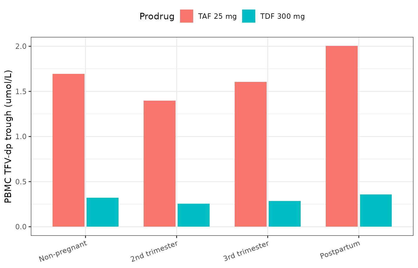
Replicates Figure 7 of Yu 2026: steady-state PBMC TFV-dp trough after 14 days of daily dosing, by prodrug and pregnancy state.
ratios <- fig7 |>
  dplyr::select("state", "Prodrug", "Cpbmc_tfvdp") |>
  tidyr::pivot_wider(names_from = "Prodrug", values_from = "Cpbmc_tfvdp") |>
  dplyr::mutate(`TAF / TDF ratio` = .data$`TAF 25 mg` / .data$`TDF 300 mg`) |>
  dplyr::rename("Pregnancy state" = "state")
knitr::kable(ratios, digits = c(0, 4, 4, 2))| Pregnancy state | TDF 300 mg | TAF 25 mg | TAF / TDF ratio |
|---|---|---|---|
| Non-pregnant | 0.3228 | 1.6944 | 5.25 |
| 2nd trimester | 0.2568 | 1.3964 | 5.44 |
| 3rd trimester | 0.2845 | 1.6048 | 5.64 |
| Postpartum | 0.3568 | 2.0030 | 5.61 |
The PBMC pool after a TAF dose is almost entirely parent-driven, which is exactly why the pregnancy effect on PBMC TFV-dp after TAF (-17.6%) tracks the bioavailability change (-17.3%) rather than the clearance change:
tafSs <- solveSemi(semiEvents("TAF", 0, 0, ndose = 14,
                              obsTimes = seq(24 * 13, 24 * 14, by = 0.25)),
                   model = tvSemi)
#> ℹ omega/sigma items treated as zero: 'etalcl', 'etalvc', 'etalka', 'etalfrac', 'etalka_tfv', 'etalcl_tfv', 'etalvc_tfv', 'etalkinf_pbmc', 'etalkinf_pbmc_tfv', 'etalkeff_pbmc'
fluxTaf <- kinfPbmc * tauAvg(tafSs, "Cc")
fluxTfv <- kinfPbmcTfv * tauAvg(tafSs, "Cc_tfv")
c(`TAF-driven fraction of PBMC influx after TAF` =
    fluxTaf / (fluxTaf + fluxTfv))
#> TAF-driven fraction of PBMC influx after TAF
#>                                    0.9836764
Concentration-time profiles
Plasma TFV and PBMC TFV-dp over 14 days (Fig. 5)
A stochastic cohort of 100 virtual women per arm (Yu 2026 used 1000; 100 is ample for the shape and keeps this vignette’s render time short).
set.seed(20260825)
NPER_ARM <- 100L

cohortSim <- function(drug) {
  lapply(seq_len(nrow(pregStates)), function(i) {
    ev <- semiEvents(drug, pregStates$EGA[i], pregStates$TPP[i],
                     ndose = 14, obsTimes = seq(0, 24 * 14, by = 6))
    ev$id <- NULL
    ev$drug <- NULL
    r <- rxode2::rxSolve(
      modSemi, ev, nSub = NPER_ARM,
      useLinCmt = FALSE, returnType = "data.frame"
    )
    r$state <- pregStates$state[i]
    r$Prodrug <- if (drug == "TAF") "TAF 25 mg" else "TDF 300 mg"
    r
  }) |> dplyr::bind_rows()
}

cohort <- dplyr::bind_rows(cohortSim("TDF"), cohortSim("TAF"))

fig5 <- cohort |>
  dplyr::select("time", "state", "Prodrug", "Cc_tfv", "Cpbmc_tfvdp") |>
  tidyr::pivot_longer(c("Cc_tfv", "Cpbmc_tfvdp"),
                      names_to = "Analyte", values_to = "conc") |>
  dplyr::mutate(Analyte = dplyr::recode(
    .data$Analyte,
    Cc_tfv = "Plasma TFV", Cpbmc_tfvdp = "PBMC TFV-dp"
  )) |>
  dplyr::group_by(.data$time, .data$state, .data$Prodrug, .data$Analyte) |>
  dplyr::summarise(median = stats::median(.data$conc), .groups = "drop")

ggplot(fig5, aes(x = time / 24, y = median, colour = state)) +
  geom_line() +
  facet_grid(Analyte ~ Prodrug, scales = "free_y") +
  labs(x = "Time (days)", y = "Median concentration (umol/L)", colour = NULL) +
  theme_bw() +
  theme(legend.position = "top")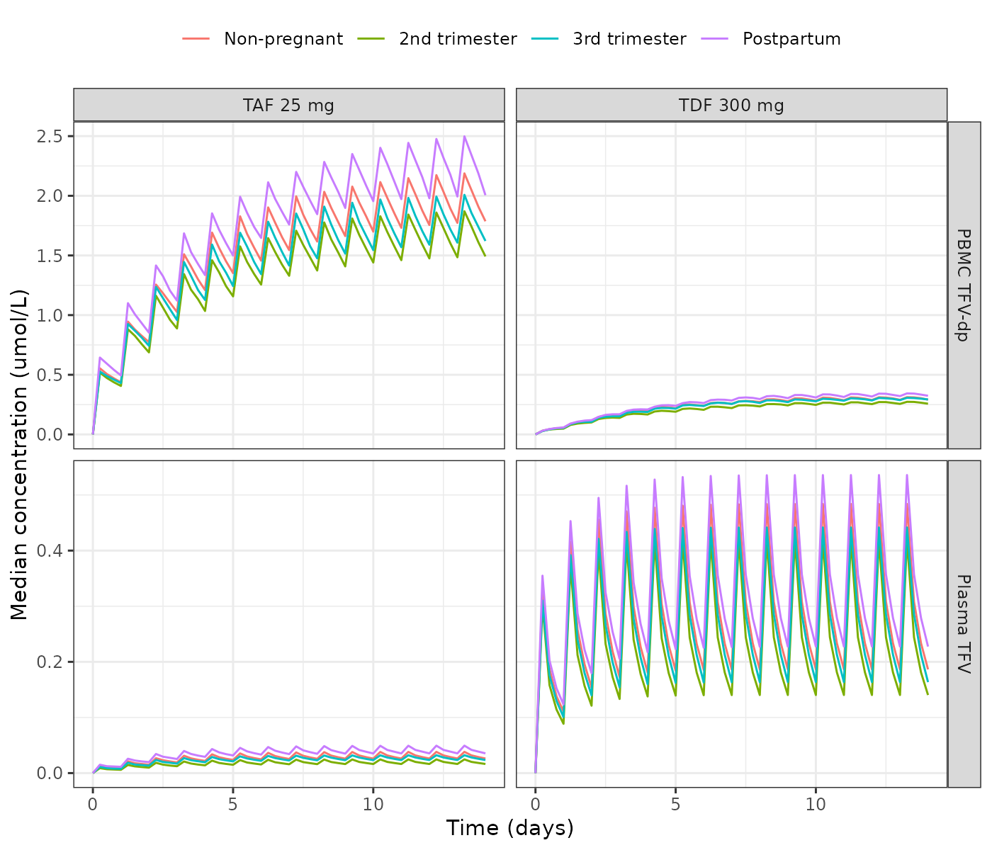
Replicates Figure 5 of Yu 2026: median simulated plasma TFV and PBMC TFV-dp over 14 days of daily dosing, by prodrug and pregnancy state (100 virtual women per arm).
DBS TFV-dp over 12 weeks (Fig. 6)
dbsProfile <- lapply(seq_len(nrow(pregStates)), function(i) {
  ev <- semiEvents("TDF", pregStates$EGA[i], pregStates$TPP[i],
                   ndose = 84, obsTimes = seq(0, 24 * 84, by = 24))
  r <- solveSemi(ev, model = tvSemi)
  r$state <- pregStates$state[i]
  r
}) |> dplyr::bind_rows()
#> ℹ omega/sigma items treated as zero: 'etalcl', 'etalvc', 'etalka', 'etalfrac', 'etalka_tfv', 'etalcl_tfv', 'etalvc_tfv', 'etalkinf_pbmc', 'etalkinf_pbmc_tfv', 'etalkeff_pbmc'
#> ℹ omega/sigma items treated as zero: 'etalcl', 'etalvc', 'etalka', 'etalfrac', 'etalka_tfv', 'etalcl_tfv', 'etalvc_tfv', 'etalkinf_pbmc', 'etalkinf_pbmc_tfv', 'etalkeff_pbmc'
#> ℹ omega/sigma items treated as zero: 'etalcl', 'etalvc', 'etalka', 'etalfrac', 'etalka_tfv', 'etalcl_tfv', 'etalvc_tfv', 'etalkinf_pbmc', 'etalkinf_pbmc_tfv', 'etalkeff_pbmc'
#> ℹ omega/sigma items treated as zero: 'etalcl', 'etalvc', 'etalka', 'etalfrac', 'etalka_tfv', 'etalcl_tfv', 'etalvc_tfv', 'etalkinf_pbmc', 'etalkinf_pbmc_tfv', 'etalkeff_pbmc'

ggplot(dbsProfile, aes(x = time / (24 * 7), y = Crbc_tfvdp, colour = state)) +
  geom_line() +
  labs(x = "Time (weeks)", y = "DBS TFV-dp (umol/L)", colour = NULL) +
  theme_bw() +
  theme(legend.position = "top")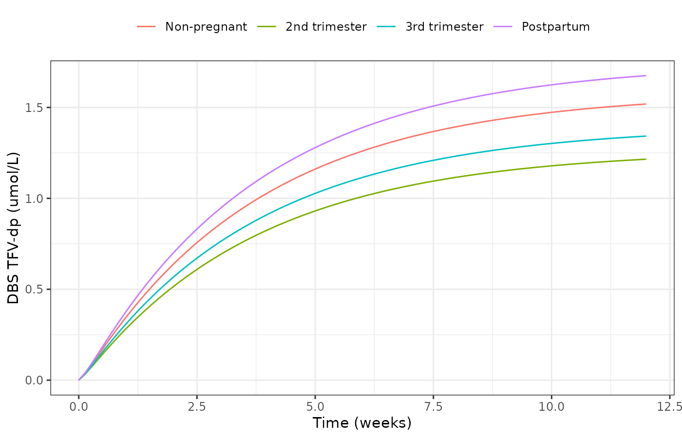
Replicates Figure 6 of Yu 2026: typical DBS TFV-dp accumulation over 12 weeks of daily TDF 300 mg, by pregnancy state.
Yu 2026 anchors this profile against observed data: “for non-pregnant women, the simulated median steady-state DBS TFV-dp concentration is consistent with fitted 50th percentiles for women with 100% adherence in the DOT-DBS study (1685 fmol/punch)”. The paper converted fmol/punch to umol/L using a red-cell volume and a per-punch cell count that it does not print, so the comparison can only be made as a dimensional consistency check: what punch red-cell volume would make the packaged model’s steady-state trough equal 1685 fmol/punch?
dbsSs <- tdf84$Crbc_tfvdp[1]                        # umol/L, non-pregnant
impliedPunchVolume_uL <- 1685e-15 / (dbsSs * 1e-6) * 1e6
c(simulated_umol_per_L = dbsSs,
  implied_punch_red_cell_volume_uL = impliedPunchVolume_uL)
#>             simulated_umol_per_L implied_punch_red_cell_volume_uL
#>                         1.518937                         1.109329
# A 3 mm DBS punch holds roughly 3 uL of whole blood, so at a normal
# haematocrit its red-cell volume is on the order of 1-1.5 uL.
stopifnot(impliedPunchVolume_uL > 0.5, impliedPunchVolume_uL < 2.5)
The implied volume is about 1.1 uL, which is what a 3 mm punch holding roughly 3 uL of whole blood contains at a normal haematocrit. This is a plausibility check on the unit chain, not a reproduction of a published number.
The two pregnancy sub-models
The standalone fits in ESM Tables S1 and S2 are the covariate-identification step: each estimates one parameter separately in each pregnancy state, with all other parameters shared. They are packaged as separate model files because they are separate NONMEM fits with their own structural parameters, not reduced views of the semi-mechanistic model.
tvTfv <- rxode2::zeroRe(modTfv)
tvTaf <- rxode2::zeroRe(modTaf)

subEvents <- function(amt, EGA, TPP, obsTimes) {
  dplyr::bind_rows(
    data.frame(time = 24 * (0:13), amt = amt, cmt = "depot", evid = 1L),
    data.frame(time = obsTimes, amt = NA_real_, cmt = "central", evid = 0L)
  ) |>
    dplyr::arrange(.data$time, dplyr::desc(.data$evid)) |>
    dplyr::mutate(EGA = EGA, TPP = TPP)
}

subProfile <- function(model, amt, label) {
  lapply(seq_len(nrow(pregStates)), function(i) {
    ev <- subEvents(amt, pregStates$EGA[i], pregStates$TPP[i],
                    seq(24 * 13, 24 * 14, by = 0.25))
    r <- rxode2::rxSolve(model, ev, useLinCmt = FALSE,
                         returnType = "data.frame")
    data.frame(time = r$time - 24 * 13, Cc = r$Cc,
               state = pregStates$state[i], Model = label)
  }) |> dplyr::bind_rows()
}

subs <- dplyr::bind_rows(
  subProfile(tvTfv, AMT_TDF, "A: plasma TFV after TDF (Table S1)"),
  subProfile(tvTaf, AMT_TAF, "B: plasma TAF (Table S2)")
)
#> ℹ omega/sigma items treated as zero: 'etalcl', 'etalka', 'etalvc'
#> ℹ omega/sigma items treated as zero: 'etalcl', 'etalka', 'etalvc'
#> ℹ omega/sigma items treated as zero: 'etalcl', 'etalka', 'etalvc'
#> ℹ omega/sigma items treated as zero: 'etalcl', 'etalka', 'etalvc'
#> ℹ omega/sigma items treated as zero: 'etalka', 'etalcl', 'etalvc'
#> ℹ omega/sigma items treated as zero: 'etalka', 'etalcl', 'etalvc'
#> ℹ omega/sigma items treated as zero: 'etalka', 'etalcl', 'etalvc'
#> ℹ omega/sigma items treated as zero: 'etalka', 'etalcl', 'etalvc'
ggplot(subs, aes(x = time, y = Cc, colour = state)) +
  geom_line() +
  facet_wrap(~Model, ncol = 1, scales = "free_y") +
  labs(x = "Time after the 14th dose (h)", y = "Concentration (umol/L)",
       colour = NULL) +
  theme_bw() +
  theme(legend.position = "top")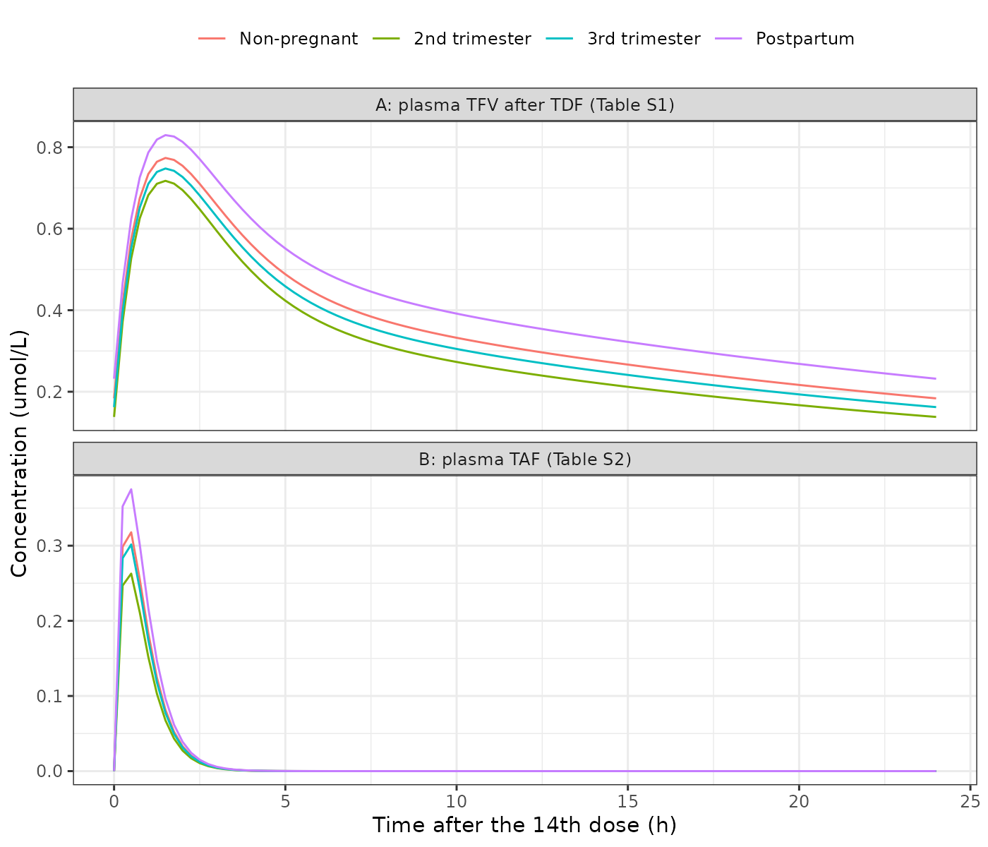
Replicates Figures 4A and 4B of Yu 2026: typical steady-state profiles from the two standalone pregnancy sub-models.
The TAF sub-model’s bioavailability estimates reproduce the percentages quoted in Results 3.2.2 exactly:
fTaf <- exp(c(
  `2nd trimester` = modTaf$theta[["lfdepot_tri2"]],
  `3rd trimester` = modTaf$theta[["lfdepot_tri3"]],
  Postpartum      = modTaf$theta[["lfdepot_pp"]]
))
tafCheck <- tibble::tibble(
  State = names(fTaf),
  `F (Table S2)` = unname(fTaf),
  `Implied change (%)` = 100 * (unname(fTaf) - 1),
  `Results 3.2.2 (%)` = c(-17.3, -5.1, 18)
)
knitr::kable(tafCheck, digits = c(0, 3, 1, 1))| State | F (Table S2) | Implied change (%) | Results 3.2.2 (%) |
|---|---|---|---|
| 2nd trimester | 0.827 | -17.3 | -17.3 |
| 3rd trimester | 0.949 | -5.1 | -5.1 |
| Postpartum | 1.180 | 18.0 | 18.0 |
The TFV sub-model’s clearances do not:
clTfv <- exp(c(
  `Non-pregnant`  = modTfv$theta[["lcl_nonpreg"]],
  `2nd trimester` = modTfv$theta[["lcl_tri2"]],
  `3rd trimester` = modTfv$theta[["lcl_tri3"]],
  Postpartum      = modTfv$theta[["lcl_pp"]]
))
tfvCheck <- tibble::tibble(
  State = names(clTfv),
  `CL/F (Table S1, L/h)` = unname(clTfv),
  `Implied change (%)` = 100 * (unname(clTfv) / clTfv[[1]] - 1),
  `Results 3.2.2 (%)` = c(NA, 24.9, 13.1, -9.3)
)
knitr::kable(tfvCheck, digits = c(0, 1, 1, 1))| State | CL/F (Table S1, L/h) | Implied change (%) | Results 3.2.2 (%) |
|---|---|---|---|
| Non-pregnant | 55.1 | 0.0 | NA |
| 2nd trimester | 65.3 | 18.5 | 24.9 |
| 3rd trimester | 59.4 | 7.8 | 13.1 |
| Postpartum | 47.6 | -13.6 | -9.3 |
Assumptions and deviations
Errata: the paper conflicts with itself on the tenofovir pregnancy effect
Results 3.2.2 states that plasma TFV apparent clearance rose 24.9% in the second trimester and 13.1% in the third and fell 9.3% postpartum. The absolute clearances printed in ESM Table S1 (55.1 / 65.3 / 59.4 / 47.6 L/h) imply +18.5% / +7.8% / -13.6% instead. The two cannot both be right.
The conflict was settled against the paper’s own simulation output
rather than by preference. Because the DBS TFV-dp pool has a 433 h
half-life, its steady-state trough is proportional to
1 / CL, so the published trough reductions invert directly
to a clearance ratio:
| Quantity | Yu 2026 reports | Implied by the text percentages | Implied by Table S1 |
|---|---|---|---|
| DBS TFV-dp trough, 2nd trimester | -20.0% (19.9-20.0) |
1/1.249 - 1 = -19.9%
|
-15.6% |
| DBS TFV-dp trough, 3rd trimester | -11.6% (11.5-11.6) |
1/1.131 - 1 = -11.6%
|
-7.2% |
| PBMC TFV-dp trough (TDF), 2nd trimester | -20.3% (19.6-21.0) | -19.9% | -15.6% |
| PBMC TFV-dp trough (TDF), 3rd trimester | -11.8% (11.3-12.2) | -11.6% | -7.2% |
The simulations therefore used the Results 3.2.2 percentages. Accordingly:
-
Yu_2026_tenofovircarries the fractional effects +0.249 / +0.131 / -0.093 oncl_tfv, which is what reproduces all ten published simulation outputs above. -
Yu_2026_tenofovir_pregnancy_tfvcarries ESM Table S1’s printed absolute clearances unchanged, because that file’s job is to reproduce Table S1.
A user who needs the two files to agree should use the semi-mechanistic model. The discrepancy is most likely a rounding or version mismatch between the covariate-model run that produced Table S1 and the text; it is not resolvable from the published material.
Other assumptions
-
Trimester boundaries. Yu 2026 reports trimester
indicator variables but never prints the gestational-age cut-offs behind
them. All three model files derive
TRI2/TRI3from the canonicalEGAcovariate using the standard obstetric boundaries (2nd trimester14 <= EGA < 28weeks, 3rd trimesterEGA >= 28weeks), andPPfromTPP > 0. The contributing IMPAACT P1026s protocol sampled at 20-26 and 30-38 weeks, both unambiguously inside these boundaries, so the choice cannot change any prediction for the studied population. No first-trimester data were available, so a record with0 < EGA < 14is scored non-pregnant. -
Postpartum window. The postpartum estimates
describe the 6-12 week window that was sampled. The models apply a
single step change for any
TPP > 0and should not be read as immediately-post-delivery values. - Molar conversions. The doses used here (473.5 umol for TDF, 52.5 umol for TAF) come from the paper’s stated 136 mg TFV equivalent and 25 mg TAF tablet divided by the standard free-base molecular weights. The paper states the conversion policy but not the molecular weights.
-
The 60 h PBMC half-life.
log(2) / Kel-PBMCis 54.6 h, not the 60 h quoted in Results 3.2.1 (and 2.5 days in the Discussion). The quoted figure is an effective half-life read from the simulated concentration-time profile, where the pool is still being fed by residual plasma drug, rather thanlog(2) / k. The packaged model carries Table 2’s rate constant, so the assertions above test the exact red-cell identity and only display the PBMC comparison. -
Bioavailability anchoring. Table 2 estimates
CL1/FandV2/F, so relative TAF bioavailability is 1 by construction in the non-pregnant state; the pregnancy effect entersf(depot)as a fractional shift from 1. The standalone TAF sub-model instead estimatesFper state with the non-pregnant value fixed to 1, which is the same parameterisation written the other way round. -
Table S2 unit labels. ESM Table S2 labels its four
Frows “(L/h)”. A bioavailability is unitless and the printed values (1, 0.827, 0.949, 1.18) reproduce the Results percentages exactly, so the unit is a copy-paste error in the source table. - Cohort size. The stochastic figure uses 100 virtual women per arm against the paper’s 1000, and the answer-key comparison uses the typical value. Neither changes a median materially.
-
Between-subject variability scale. Table 2 and ESM
Tables S1/S2 report BSV as
%CVfor the exponential model of Methods 2.4.1, so everyetavariance isomega^2 = log(CV^2 + 1). - No residual-error correlation. The paper reports one residual model per analyte and no correlation between them; the model files reproduce that.
Naming decisions
The PBMC influx / efflux rate constants had no registered equivalent.
The lkinf_pbmc (parent-driven, plasma TAF),
lkinf_pbmc_tfv (plasma-TFV-driven) and
lkeff_pbmc family was ratified for this extraction as the
PBMC parallel of the existing lkinf_rbc /
lkeff_rbc family, and registered in
inst/references/parameter-names.md. The red-cell pair keeps
its registered bare names even though this file’s dosed parent is TAF
while the red-cell influx is driven by plasma TFV, because the pool has
a single influx and forking to a suffixed name away from an existing
canonical would defeat reuse. The paper’s FTFV,
Ffast and Kslow map onto the registered
canonicals fm, frac and ktr
respectively.