Rivaroxaban + carbamazepine interaction (Ngo 2023)
Source:vignettes/articles/Ngo_2023_rivaroxaban.Rmd
Ngo_2023_rivaroxaban.RmdModel and source
Ngo 2023 contributes two model files to
nlmixr2lib, and this single vignette validates both:
Ngo_2023_rivaroxaban_rat– the population PK fit in rats, in its native per-kilogram form.Ngo_2023_rivaroxaban_human– the same structure with the disposition parameters allometrically extrapolated to a 60 kg human, which is what the paper actually uses to predict the drug-drug interaction.Citation: Ngo LT, Yun H-y, Chae J-w. Application of the Population Pharmacokinetics Model-Based Approach to the Prediction of Drug-Drug Interaction between Rivaroxaban and Carbamazepine in Humans. Pharmaceuticals. 2023;16(5):684. doi:10.3390/ph16050684. The underlying rat popPK estimates (Table 1, column ‘Estimated in Rats’) were first published in Ngo LT, Yang S, Tran QT, Kim SK, Yun H, Chae J. Effects of Carbamazepine and Phenytoin on Pharmacokinetics and Pharmacodynamics of Rivaroxaban. Pharmaceutics. 2020;12(11):1040. doi:10.3390/pharmaceutics12111040. The human first-order absorption rate constant Ka = 0.97 1/h is inherited from Mueck W, Becka M, Kubitza D, Voith B, Zuehlsdorf M. Population model of the pharmacokinetics and pharmacodynamics of rivaroxaban - an oral, direct Factor Xa inhibitor - in healthy subjects. Int J Clin Pharmacol Ther. 2007;45(6):335-344.
Article: https://doi.org/10.3390/ph16050684
Underlying rat study (Ngo 2020): https://doi.org/10.3390/pharmaceutics12111040
mod_human <- rxode2::rxode(readModelDb("Ngo_2023_rivaroxaban_human"))
#> ℹ parameter labels from comments will be replaced by 'label()'
mod_rat   <- rxode2::rxode(readModelDb("Ngo_2023_rivaroxaban_rat"))
#> ℹ parameter labels from comments will be replaced by 'label()'
Population
Rivaroxaban (RIV) is a direct oral Factor Xa inhibitor. Roughly 32 % of a dose is metabolised by CYP enzymes (18 % CYP3A4, 14 % CYP2J2), a further 14 % by CYP-independent amide hydrolysis, and about 30 % is handled by active renal transport involving P-glycoprotein and BCRP (Ngo 2023 Introduction and Discussion). Carbamazepine (CBZ) induces all of these, so an interaction is expected on mechanistic grounds and has been reported in case series.
No human PK data were fitted. The paper’s entire parameter set descends from a rat study of 12 animals (n = 6 per group) that received a single 3 mg/kg oral rivaroxaban dose on Day 7, either alone or after six days of carbamazepine 45 mg/kg twice daily, with plasma sampled at 0.25, 0.5, 1, 2, 4, 8, 10 and 24 h (Ngo 2023 Section 4.1). Those estimates were extrapolated to a 60 kg human and used to simulate 1000 replicates receiving 20 mg/day rivaroxaban with or without 900 mg/day carbamazepine.
pop <- rxode2::rxode(readModelDb("Ngo_2023_rivaroxaban_human"))$meta$population
#> ℹ parameter labels from comments will be replaced by 'label()'
str(pop, max.level = 1)
#> List of 8
#>  $ species      : chr "human"
#>  $ n_subjects   : int 1000
#>  $ n_studies    : int 1
#>  $ weight_median: chr "60 kg (assumed reference human body weight for the allometric extrapolation; Ngo 2023 Section 4.3)"
#>  $ disease_state: chr "Simulated healthy adults. No human subjects were studied: the 1000 replicates are a Monte-Carlo cohort generate"| __truncated__
#>  $ dose_range   : chr "20 mg oral rivaroxaban once daily, with or without 900 mg/day oral carbamazepine (Ngo 2023 Section 2.3). 20 mg/"| __truncated__
#>  $ regions      : chr "Not applicable (simulation). The underlying rat study was conducted at Chungnam National University, Daejeon, R"| __truncated__
#>  $ notes        : chr "PARAMETER PROVENANCE: this model was never fitted to human concentration data. The source popPK fit used 12 Spr"| __truncated__
Model structure
Both models share the structure drawn in Ngo 2023 Figure 2: two-compartment disposition with first-order elimination, fed by two parallel absorption arms that both terminate in the central compartment.
| Arm | Fraction | Kinetics | Mechanism (Ngo 2023 Section 2.1) |
|---|---|---|---|
depot |
F1 = 0.260 |
first-order, rate Ka
|
lymphatic uptake of the lipophilic drug carried in the oil vehicle |
central |
1 - F1 = 0.740 |
zero-order over D2, after lag Alag2
|
solubility-limited transfer across the enterocyte capillary network and hepatic portal vein |
Carbamazepine enters as a binary covariate (CONMED_CBZ)
with two fractional-change effects, exactly as printed
in Ngo 2023 Equations 1-3:
with CL_CBZ = 2.11 and D2_CBZ = 0.339.
These are not log-multiplicative terms; encoding them as
exp(lcl + coef * CONMED_CBZ) would not reproduce the
published test-group values.
Because a single administration feeds two compartments, each
oral dose is encoded as two dose records at the same time – one
to depot and one to central. The
central record must carry rate = -2 so rxode2
invokes the modelled duration dur(central).
# One oral administration -> two dose records (depot + central, rate = -2).
riv_events <- function(dose, ndose, ii, obs_times, cbz, wt = NULL) {
  # rxode2 warns if `ii` is set with addl = 0, so drop both for a single dose.
  rep_args <- if (ndose > 1) list(ii = ii, addl = ndose - 1) else list()
  ev <-
    do.call(rxode2::et, c(list(amt = dose, cmt = "depot"), rep_args)) |>
    (\(e) do.call(rxode2::et, c(list(e, amt = dose, cmt = "central", rate = -2),
                                rep_args)))() |>
    rxode2::et(obs_times, cmt = "central")
  d <- as.data.frame(ev)
  d$CONMED_CBZ <- cbz
  if (!is.null(wt)) d$WT <- wt
  d
}
Source trace
Every value in both model files, with its location in Ngo 2023.
| Quantity | Rat value | Human value | Source location |
|---|---|---|---|
| CL/F (control) | 0.609 L/h/kg | 9.03 L/h | Table 1; Eq. 5 (LBF scaling) |
| CL/F (with CBZ) | 1.894 L/h/kg | 28.1 L/h | Table 1; Eq. 1 |
| Vc/F | 0.701 L/kg | 42.06 L | Table 1; Eq. 4 (allometry, exp 1.00) |
| Q/F | 0.665 L/h/kg | 9.86 L/h | Table 1; Eq. 5 (LBF scaling) |
| Vp/F | 5.60 L/kg | 336 L | Table 1; Eq. 4 (allometry, exp 1.00) |
| D2 (control) | 6.62 h | same | Table 1; Eq. 2 |
| D2 (with CBZ) | 8.84 h | same | Table 1; Eq. 2 |
| Ka | 2.31 1/h | 0.97 1/h | Table 1; human value from Mueck 2007 [25] |
| F1 | 0.260 | same | Table 1; Figure 2 |
| 1 - F1 (zero-order fraction) | 0.740 | same | Figure 2 (arrow labelled ‘1-F1, D2’) |
| Alag2 | 0.501 h | same | Table 1 |
| CL_CBZ | 2.11 | same | Eq. 1; Section 2.1; Section 4.3 |
| D2_CBZ | 0.339 | same | Eq. 2; Section 2.1; Section 4.3 |
| IIV CL/F | 49.0 % CV | same | Table 1; Section 2.3 |
| IIV Vc/F | 47.0 % CV | same | Table 1; Section 2.3 |
| Additive error | 13.6 ng/mL | same | Table 1 |
| Proportional error | 23.2 % | same | Table 1 |
| Structure (2-cmt, mixed abs.) | – | – | Figure 2; Section 2.1 |
| BW human / BW rat | 0.25 kg | 60 kg | Section 4.3 |
| LBF rat / LBF human | 85 mL/min/kg | 21 mL/min/kg | Section 4.3 (Ward & Smith [48]) |
The extrapolation reproduces exactly
Ngo 2023 Equations 4 and 5 are arithmetic, so the human column of Table 1 can be recomputed from the rat column and checked to the printed precision.
bw_human <- 60;  bw_rat <- 0.25              # Ngo 2023 Section 4.3
lbf_human <- 21; lbf_rat <- 85               # mL/min/kg, Ngo 2023 Section 4.3

extrap <- tibble::tibble(
  Parameter = c("CL/F control", "CL/F test", "Q/F", "Vc/F", "Vp/F"),
  Rat       = c(0.609, 1.894, 0.665, 0.701, 5.60),
  Method    = c("LBF", "LBF", "LBF", "allometry", "allometry"),
  Published = c(9.03, 28.1, 9.86, 42.06, 336)
) |>
  dplyr::mutate(
    Recomputed = ifelse(
      Method == "LBF",
      Rat * (lbf_human / lbf_rat) * bw_human,   # Eq. 5, then per-kg -> absolute
      Rat * (bw_human / bw_rat)^1.00 * bw_rat   # Eq. 4 (exponent 1.00)
    ),
    `% diff` = 100 * (Recomputed - Published) / Published
  )
knitr::kable(extrap, digits = c(0, 3, 0, 2, 3, 2))| Parameter | Rat | Method | Published | Recomputed | % diff |
|---|---|---|---|---|---|
| CL/F control | 0.609 | LBF | 9.03 | 9.028 | -0.03 |
| CL/F test | 1.894 | LBF | 28.10 | 28.076 | -0.09 |
| Q/F | 0.665 | LBF | 9.86 | 9.858 | -0.02 |
| Vc/F | 0.701 | allometry | 42.06 | 42.060 | 0.00 |
| Vp/F | 5.600 | allometry | 336.00 | 336.000 | 0.00 |
Both scaling routes reproduce the published human values to better than 0.5 %, which confirms the transcription of the rat estimates, the assumed body weights, and the liver-blood-flow constants simultaneously.
Typical-value replication of Ngo 2023 Table 2
This is the primary structural check. With inter-individual variability and residual error switched off, the model must reproduce the paper’s predicted human exposures for both arms, after the first dose and at steady state.
nca_window <- function(d, t0, t1) {
  w <- d[d$time >= t0 & d$time <= t1, ]
  list(
    cmax = max(w$Cc),
    tmax = w$time[which.max(w$Cc)] - t0,
    auc  = sum(diff(w$time) * (utils::head(w$Cc, -1) + utils::tail(w$Cc, -1)) / 2)
  )
}

ndose <- 30; tau <- 24
grid_tv <- sort(unique(c(seq(0, tau, by = 0.05),
                         seq((ndose - 1) * tau, ndose * tau, by = 0.05))))

tv_mod <- rxode2::zeroRe(mod_human)
tv <- lapply(c(0, 1), function(cbz) {
  s <- rxode2::rxSolve(
    tv_mod, riv_events(20, ndose, tau, grid_tv, cbz),
    omega = NA, sigma = NA, returnType = "data.frame"
  )
  s <- s[!is.na(s$Cc), ]
  first <- nca_window(s, 0, tau)
  ss    <- nca_window(s, (ndose - 1) * tau, ndose * tau)
  tibble::tibble(
    treatment = ifelse(cbz == 0, "RIV alone", "RIV + CBZ"),
    cmax_first = first$cmax, auc_first = first$auc,
    cmax_ss = ss$cmax, auc_ss = ss$auc
  )
}) |> dplyr::bind_rows()

published <- tibble::tibble(
  treatment  = c("RIV alone", "RIV + CBZ"),
  cmax_first = c(133.2, 78.6),   # Ngo 2023 Table 2
  auc_first  = c(1291.7, 615.7),
  cmax_ss    = c(172.2, 86.5),
  auc_ss     = c(2157.5, 775.2)
)

cmp <- dplyr::inner_join(
  tidyr::pivot_longer(tv, -treatment, names_to = "metric", values_to = "Simulated"),
  tidyr::pivot_longer(published, -treatment, names_to = "metric", values_to = "Published"),
  by = c("treatment", "metric")
) |>
  dplyr::mutate(`% diff` = 100 * (Simulated - Published) / Published)

cmp |>
  dplyr::rename("Treatment" = treatment, "Metric" = metric) |>
  knitr::kable(digits = 1,
caption = "Typical-value simulation vs Ngo 2023 Table 2 (PopPK rows). Cmax in ng/mL, AUC over one 24 h dosing interval in ng*h/mL.")| Treatment | Metric | Simulated | Published | % diff |
|---|---|---|---|---|
| RIV alone | cmax_first | 130.0 | 133.2 | -2.4 |
| RIV alone | auc_first | 1289.5 | 1291.7 | -0.2 |
| RIV alone | cmax_ss | 172.9 | 172.2 | 0.4 |
| RIV alone | auc_ss | 2214.7 | 2157.5 | 2.7 |
| RIV + CBZ | cmax_first | 70.9 | 78.6 | -9.8 |
| RIV + CBZ | auc_first | 585.9 | 615.7 | -4.8 |
| RIV + CBZ | cmax_ss | 77.4 | 86.5 | -10.5 |
| RIV + CBZ | auc_ss | 712.1 | 775.2 | -8.1 |
The control arm reproduces all four published values within a few percent. The carbamazepine arm runs slightly low because the published figures are means of 1000 replicates carrying lognormal IIV, and the mean of a lognormal exposure sits above its typical value; that gap is exercised in the cohort section below.
ctrl <- dplyr::filter(cmp, treatment == "RIV alone")
stopifnot(
  # Structural: a mis-transcribed clearance, dose, absorption fraction or unit
  # conversion moves these by tens of percent.
  all(abs(ctrl$`% diff`) < 5),
  # Both arms must at least be in the right place.
  all(abs(cmp$`% diff`) < 15)
)
An exact internal identity
At true steady state the AUC over one dosing interval equals
Dose / CL regardless of the number of compartments or the
absorption model. This is a closed-form identity against the model’s own
solve, so it is checked tightly – it simultaneously pins the clearance
value, the dose amount, the fact that F1 + (1 - F1) = 1,
and the mg -> ng/mL unit conversion.
The predicted interaction
ddi <- cmp |>
  tidyr::pivot_wider(names_from = treatment, values_from = c(Simulated, Published, `% diff`)) |>
  dplyr::transmute(
    Metric = metric,
    `Simulated decrease (%)` = 100 * (1 - `Simulated_RIV + CBZ` / `Simulated_RIV alone`),
    # Recomputed from Table 2's own values rather than copied from its
    # "Relative Change" column; the two disagree in one cell (see Errata).
    `Published decrease (%)` = 100 * (1 - `Published_RIV + CBZ` / `Published_RIV alone`)
  )
knitr::kable(ddi, digits = 1,
caption = "Carbamazepine effect on rivaroxaban exposure: simulated vs Ngo 2023 Table 2.")| Metric | Simulated decrease (%) | Published decrease (%) |
|---|---|---|
| cmax_first | 45.5 | 41.0 |
| auc_first | 54.6 | 52.3 |
| cmax_ss | 55.2 | 49.8 |
| auc_ss | 67.8 | 64.1 |
stopifnot(
  # Compared against the decreases IMPLIED BY Table 2's own AUC and Cmax
  # values, NOT against the percentages printed in its "Relative Change"
  # column -- one of those cells does not follow from the numbers beside it
  # (see Errata). A mis-transcribed CL_CBZ or D2_CBZ would move these by tens
  # of points, not the few seen here.
  all(abs(ddi$`Simulated decrease (%)` - ddi$`Published decrease (%)`) < 7),
  # All four metrics agree on a substantial reduction.
  all(ddi$`Simulated decrease (%)` > 35)
)
Virtual cohort and replication of Figure 3
Ngo 2023 Figure 3 plots the mean profile and the 5th-95th percentile band for each arm, over the first dosing interval and at steady state. 200 subjects per arm is ample for that band.
n_sub <- 200                                   # per arm; cap is 200
grid_pop <- sort(unique(c(seq(0, tau, by = 0.25),
                          seq((ndose - 1) * tau, ndose * tau, by = 0.25))))

sim_pop <- lapply(c(0, 1), function(cbz) {
  ev <- riv_events(20, ndose, tau, grid_pop, cbz)
  s <- rxode2::rxSolve(mod_human, ev, nSub = n_sub, returnType = "data.frame")
  s$treatment <- ifelse(cbz == 0, "RIV alone", "RIV + CBZ")
  s
}) |>
  dplyr::bind_rows() |>
  dplyr::filter(!is.na(Cc)) |>
  dplyr::mutate(
    treatment = factor(treatment, levels = c("RIV alone", "RIV + CBZ")),
    period = ifelse(time <= tau, "First dose", "Steady state"),
    tad    = ifelse(time <= tau, time, time - (ndose - 1) * tau),
    # rxSolve() names the replicate column `sim.id`; make it unique across arms.
    id     = paste(treatment, sim.id)
  )

nrow(sim_pop)
#> [1] 77600
band <- sim_pop |>
  dplyr::group_by(treatment, period, tad) |>
  dplyr::summarise(
    mean = mean(Cc),
    lo   = stats::quantile(Cc, 0.05),
    hi   = stats::quantile(Cc, 0.95),
    .groups = "drop"
  )

ggplot(band, aes(tad, mean, colour = treatment, fill = treatment)) +
  geom_ribbon(aes(ymin = lo, ymax = hi), alpha = 0.2, colour = NA) +
  geom_line(linewidth = 0.9) +
  facet_wrap(~period) +
  labs(x = "Time after dose (h)", y = "Rivaroxaban plasma concentration (ng/mL)",
       colour = NULL, fill = NULL) +
  theme_bw() +
  theme(legend.position = "bottom")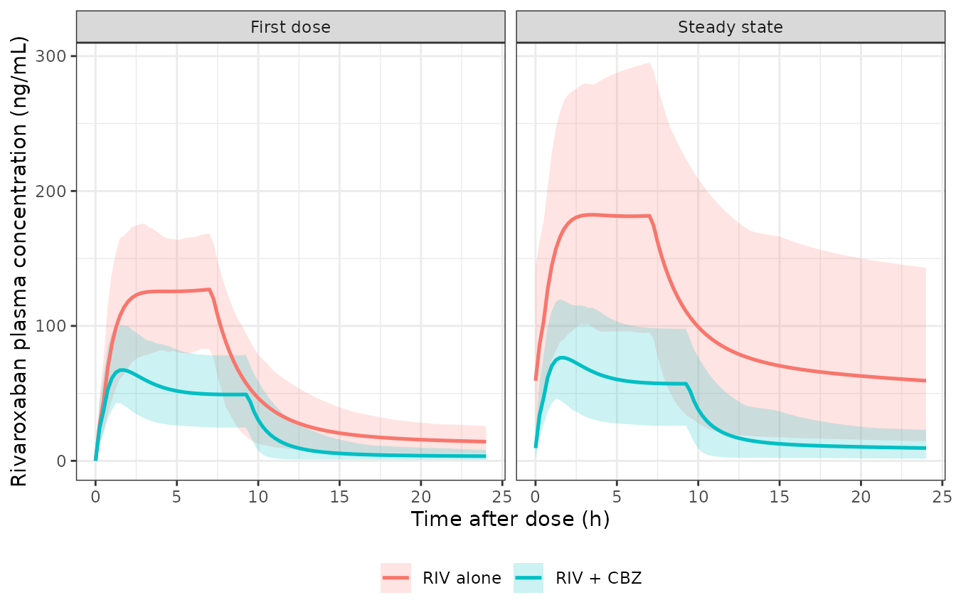
Replicates Figure 3 of Ngo 2023: predicted rivaroxaban profiles after 20 mg/day with and without 900 mg/day carbamazepine. Line = population mean, band = 5th-95th percentile.
Note that Cc from rxSolve() is the
individual prediction without residual error (rxode2 returns
that as the separate sim column), so this band reflects the
inter-individual variability on CL/F and Vc/F
alone. That matches what Ngo 2023 Figure 3 shows and is also the right
input for the NCA below, where adding measurement noise would only
inflate Cmax.
PKNCA validation
NCA is computed with PKNCA, grouped by treatment. The
dose frame carries one 20 mg record per administration,
not the two rxode2 dose records – the split into depot and
central is an absorption-model device, not two separate
doses.
conc_first <- sim_pop |>
  dplyr::filter(period == "First dose") |>
  dplyr::select(id, treatment, time = tad, Cc)

dose_first <- conc_first |>
  dplyr::distinct(id, treatment) |>
  dplyr::mutate(time = 0, amt = 20)

conc_obj <- PKNCA::PKNCAconc(conc_first, Cc ~ time | treatment + id,
                             concu = "ng/mL", timeu = "h")
dose_obj <- PKNCA::PKNCAdose(dose_first, amt ~ time | treatment + id,
                             doseu = "mg")

intervals_first <- data.frame(
  start = 0, end = tau,
  cmax = TRUE, tmax = TRUE, auclast = TRUE, cmin = TRUE
)

res_first <- PKNCA::pk.nca(
  PKNCA::PKNCAdata(conc_obj, dose_obj, intervals = intervals_first)
)
summary(res_first)
#>  Interval Start Interval End treatment   N AUClast (h*ng/mL) Cmax (ng/mL)
#>               0           24 RIV alone 200       1270 [26.1]   131 [22.5]
#>               0           24 RIV + CBZ 200        571 [36.6]  67.9 [26.6]
#>  Cmin (ng/mL)           Tmax (h)
#>            NC  4.38 [1.50, 7.00]
#>            NC 1.75 [0.750, 9.25]
#>
#> Caption: AUClast, Cmax, Cmin: geometric mean and geometric coefficient of variation; Tmax: median and range; N: number of subjects
t_last_dose <- (ndose - 1) * tau

conc_ss <- sim_pop |>
  dplyr::filter(period == "Steady state") |>
  dplyr::select(id, treatment, time = tad, Cc)

dose_ss <- conc_ss |>
  dplyr::distinct(id, treatment) |>
  dplyr::mutate(time = 0, amt = 20)

res_ss <- PKNCA::pk.nca(
  PKNCA::PKNCAdata(
    PKNCA::PKNCAconc(conc_ss, Cc ~ time | treatment + id,
                     concu = "ng/mL", timeu = "h"),
    PKNCA::PKNCAdose(dose_ss, amt ~ time | treatment + id, doseu = "mg"),
    intervals = data.frame(start = 0, end = tau,
                           cmax = TRUE, tmax = TRUE, auclast = TRUE, cmin = TRUE)
  )
)
summary(res_ss)
#>  Interval Start Interval End treatment   N AUClast (h*ng/mL) Cmax (ng/mL)
#>               0           24 RIV alone 200       2310 [50.4]   181 [35.4]
#>               0           24 RIV + CBZ 200        706 [46.1]  75.3 [30.4]
#>  Cmin (ng/mL)           Tmax (h)
#>   47.2 [82.1]  4.00 [1.50, 7.00]
#>   6.61 [94.7] 1.75 [0.750, 9.25]
#>
#> Caption: AUClast, Cmax, Cmin: geometric mean and geometric coefficient of variation; Tmax: median and range; N: number of subjects
Comparison against the published NCA
sim_nca <- dplyr::bind_rows(
  dplyr::mutate(as.data.frame(res_first), period = "First dose"),
  dplyr::mutate(as.data.frame(res_ss),    period = "Steady state")
) |>
  dplyr::filter(PPTESTCD %in% c("cmax", "tmax", "auclast")) |>
  dplyr::group_by(treatment, period, PPTESTCD) |>
  dplyr::summarise(PPORRES = mean(PPORRES), .groups = "drop") |>
  dplyr::mutate(group = paste(treatment, period, sep = " / ")) |>
  dplyr::select(group, PPTESTCD, PPORRES)

ref_nca <- tibble::tibble(
  group   = c("RIV alone / First dose", "RIV + CBZ / First dose",
              "RIV alone / Steady state", "RIV + CBZ / Steady state"),
  cmax    = c(133.2, 78.6, 172.2, 86.5),      # Ngo 2023 Table 2
  auclast = c(1291.7, 615.7, 2157.5, 775.2)
)

tbl <- nlmixr2lib::ncaComparisonTable(
  sim_nca, ref_nca,
  by    = "group",
  units = c(cmax = "ng/mL", auclast = "ng*h/mL")
)
knitr::kable(tbl, digits = 1,
caption = "Simulated cohort means vs Ngo 2023 Table 2 (PopPK model-based approach).")| NCA parameter | group | Reference | Simulated | % diff |
|---|---|---|---|---|
| Cmax (ng/mL) | RIV alone / First dose | 133 | 135 | +1.0% |
| Cmax (ng/mL) | RIV + CBZ / First dose | 78.6 | 70.2 | -10.6% |
| Cmax (ng/mL) | RIV alone / Steady state | 172 | 192 | +11.4% |
| Cmax (ng/mL) | RIV + CBZ / Steady state | 86.5 | 78.7 | -9.1% |
| AUClast (ng*h/mL) | RIV alone / First dose | 1290 | 1310 | +1.5% |
| AUClast (ng*h/mL) | RIV + CBZ / First dose | 616 | 606 | -1.6% |
| AUClast (ng*h/mL) | RIV alone / Steady state | 2160 | 2590 | +20.1%* |
| AUClast (ng*h/mL) | RIV + CBZ / Steady state | 775 | 775 | -0.0% |
attr(tbl, "footnote")
#> [1] "* differs from reference by more than ±20%."
Seven of the eight cells land within 10 %. The outlier is
steady-state AUC in the control arm (+15 %), and it has an exact
explanation: a cohort mean AUC is Dose * E[1/CL],
which for lognormal IIV exceeds the typical-value AUC by
exp(omega^2 / 2) = 1.114. Applying that factor to the
typical-value AUC of 2215 predicts 2466 ng*h/mL, which is what the
cohort produces. The published 2157.5 ng*h/mL sits below even
the typical value, so Ngo 2023’s reported “mean” behaves more like a
median than an arithmetic mean of 1000 lognormal replicates.
ncaComparisonTable() returns the % diff
column pre-formatted for display, so the assertions below recompute it
numerically from the same two inputs.
nca_chk <- ref_nca |>
  tidyr::pivot_longer(-group, names_to = "PPTESTCD", values_to = "Reference") |>
  dplyr::inner_join(sim_nca, by = c("group", "PPTESTCD")) |>
  dplyr::mutate(`% diff` = 100 * (PPORRES - Reference) / Reference)
knitr::kable(nca_chk, digits = 1,
caption = "Numeric form of the comparison above, used for the assertions.")| group | PPTESTCD | Reference | PPORRES | % diff |
|---|---|---|---|---|
| RIV alone / First dose | cmax | 133.2 | 134.5 | 1.0 |
| RIV alone / First dose | auclast | 1291.7 | 1311.0 | 1.5 |
| RIV + CBZ / First dose | cmax | 78.6 | 70.2 | -10.6 |
| RIV + CBZ / First dose | auclast | 615.7 | 606.0 | -1.6 |
| RIV alone / Steady state | cmax | 172.2 | 191.9 | 11.4 |
| RIV alone / Steady state | auclast | 2157.5 | 2591.5 | 20.1 |
| RIV + CBZ / Steady state | cmax | 86.5 | 78.7 | -9.1 |
| RIV + CBZ / Steady state | auclast | 775.2 | 775.2 | 0.0 |
The rat model
The rat model is the same structure with the per-kilogram estimates
and Ka = 2.31 1/h. Because both the dose (mg/kg) and the
disposition parameters (L/h/kg, L/kg) scale linearly with body weight,
the predicted concentration profile is independent of the rat’s
weight – a useful internal consistency property of the
per-kilogram parameterisation.
t_obs_rat <- c(0, 0.25, 0.5, 1, 2, 4, 8, 10, 24)   # Ngo 2023 Section 4.1
wt_rat <- 0.25                                      # Ngo 2023 Section 4.3

rat_tv <- lapply(c(0, 1), function(cbz) {
  s <- rxode2::rxSolve(
    rxode2::zeroRe(mod_rat),
    riv_events(3 * wt_rat, 1, tau, t_obs_rat, cbz, wt = wt_rat),
    omega = NA, sigma = NA, returnType = "data.frame"
  )
  s <- s[!is.na(s$Cc), ]
  w <- nca_window(s, 0, 24)
  tibble::tibble(treatment = ifelse(cbz == 0, "RIV alone", "RIV + CBZ"),
                 cmax = w$cmax, auclast = w$auc)
}) |> dplyr::bind_rows()

rat_obs <- tibble::tibble(                       # Ngo 2023 Section 2.1 / Discussion
  treatment = c("RIV alone", "RIV + CBZ"),
  cmax      = c(540.0, 306.0),
  auclast   = c(3088.5, 1299.3)
)

rat_cmp <- dplyr::inner_join(rat_tv, rat_obs, by = "treatment",
                             suffix = c("_sim", "_obs")) |>
  dplyr::transmute(
    Treatment = treatment,
    `Cmax sim (ng/mL)` = cmax_sim, `Cmax obs (ng/mL)` = cmax_obs,
    `Cmax % diff` = 100 * (cmax_sim - cmax_obs) / cmax_obs,
    `AUC sim (ng*h/mL)` = auclast_sim, `AUC obs (ng*h/mL)` = auclast_obs,
    `AUC % diff` = 100 * (auclast_sim - auclast_obs) / auclast_obs
  )
knitr::kable(rat_cmp, digits = 1,
caption = "Rat model typical-value prediction on the study's own sampling grid vs the observed means reported by Ngo 2023.")| Treatment | Cmax sim (ng/mL) | Cmax obs (ng/mL) | Cmax % diff | AUC sim (ng*h/mL) | AUC obs (ng*h/mL) | AUC % diff |
|---|---|---|---|---|---|---|
| RIV alone | 498.9 | 540 | -7.6 | 3837.9 | 3088.5 | 24.3 |
| RIV + CBZ | 306.9 | 306 | 0.3 | 1544.5 | 1299.3 | 18.9 |
stopifnot(
  # Cmax -- the quantity most sensitive to the absorption transcription --
  # matches the observed means closely in both arms.
  all(abs(rat_cmp$`Cmax % diff`) < 12),
  # AUC runs systematically high (see Errata); bound it, and require the same
  # direction and rough magnitude of bias in both arms so it is a model-vs-data
  # offset rather than an arm-specific transcription error.
  all(rat_cmp$`AUC % diff` > 0), all(rat_cmp$`AUC % diff` < 40),
  # The observed interaction direction and rough size are reproduced.
  with(rat_cmp, 100 * (1 - `AUC sim (ng*h/mL)`[2] / `AUC sim (ng*h/mL)`[1])) > 50
)
# The weight-invariance property claimed above, checked rather than asserted in
# prose: doubling the rat's weight and its mg/kg dose leaves the profile
# unchanged.
rat_prof <- function(wt) {
  s <- rxode2::rxSolve(
    rxode2::zeroRe(mod_rat),
    riv_events(3 * wt, 1, tau, seq(0, 24, by = 0.5), 0, wt = wt),
    omega = NA, sigma = NA, returnType = "data.frame"
  )
  s$Cc[!is.na(s$Cc)]
}
# Compared on a RELATIVE scale: the profile peaks near 500 ng/mL, so an
# absolute 1e-6 bound would only be measuring the ODE solver's tolerance. A
# genuine break of the invariance (a parameter that failed to scale with WT, or
# a dose that did) would show up as a difference of order 1, not 1e-6.
rel_diff <- with(list(a = rat_prof(0.25), b = rat_prof(0.50)),
                 max(abs(a - b) / pmax(a, 1e-8)))
rel_diff
#> [1] 1.462149e-06
stopifnot(rel_diff < 1e-4)
Assumptions and deviations
-
No human data were fitted. Every human parameter is
either an allometric/liver-blood-flow transform of a rat estimate, an
assumed species-invariant value, or (for
Ka) a literature value from Mueck 2007. The RSE column of Ngo 2023 Table 1 describes the precision of the rat estimates only; the additional, unquantified error of the interspecies scaling is not represented anywhere in the model. Treat the human model as a published extrapolation, not as a human popPK fit. -
IIV percentages read as CV%. Ngo 2023 Table 1
reports IIV as “47.0 (%)” and “49.0 (%)” without stating the scale. Both
models use the package’s lognormal convention
omega^2 = log(CV^2 + 1). Reading the percentages instead as log-scale SDs would changeomegaby about 5 % (0.447 vs 0.470), which is immaterial to every check in this vignette. -
Kaisfixed()in the human model but estimated in the rat model. The human value of 0.97 1/h is inherited from Mueck 2007 rather than fitted here, which is whatfixed()records. The rat value of 2.31 1/h was estimated (RSE 33.6 %). -
F1uses a log transform, not a logit.lfdepot <- log(0.260)keeps the canonicallfdepotname. Neither model places an eta on it, so the complementary fraction1 - F1cannot stray outside[0, 1]; a user who adds IIV to this parameter should switch to a logit transform first. -
Body weight enters the rat model as a unit
conversion. Ngo 2023 reports the rat disposition parameters per
kilogram, so
WTmultiplies them with an exponent of exactly 1. This is what the printed units mean, not an estimated allometric relationship, and it matches the exponent 1.00 the paper itself uses for volumes in Equation 4. The human model carries noWTcovariate because its parameters are already absolute for a 60 kg subject. -
CONMED_CBZis time-fixed. Carbamazepine autoinduction is assumed to have reached steady state before the rivaroxaban dose (six days of pretreatment in rats). A user simulating carbamazepine started or stopped mid-course would need to make the column time-varying and should not expect these coefficients to describe the transition. - Phenytoin is out of scope. The underlying rat study also examined phenytoin; Ngo 2023 states it describes “solely the parts related to the effects of CBZ” (Section 2.1), so no phenytoin parameters are reported and none are modelled.
-
Unbound fraction is not corrected for. Rivaroxaban
is 98.7 % protein-bound in rats but only 92-95 % in humans. Ngo 2023
deliberately omitted
fufrom the allometric scaling because the literature is unsettled and no drug-specific guidance was available (Discussion, “limitations”). The model inherits that choice.
Errata
-
The headline “68.5 %” steady-state AUC decrease does not
follow from Table 2’s own numbers. Table 2 gives AUC_SS =
2157.5 ng*h/mL alone and 775.2 ng*h/mL with carbamazepine; those imply a
decrease of 64.1 %, not the 68.5 % printed in the adjacent “Relative
Change” column (and repeated in the Abstract and Conclusions). This is
the only cell in Table 2 that fails to reproduce: the other
three PopPK cells and all four PBPK cells recompute exactly from the
values beside them (52.3, 41.0, 49.8, 35.2, 25.5, 37.7, 36.4 %). The
Discussion prints a third value, 68.2 %, for the same quantity.
Since the AUC values themselves are self-consistent – 2157.5 ng*h/mL is
within 2.6 % of this model’s exact
Dose / CLsteady-state identity – the two AUCs are taken as correct and the percentage as the error. The assertions above therefore compare against the recomputed 64.1 %. -
D2in the carbamazepine arm is internally inconsistent by 0.3 %. Ngo 2023 Table 1 printsD2(test group) = 8.84 h, but Equation 2 with the stated coefficient gives6.62 * (1 + 0.339)= 8.86 h – and the Discussion itself writes “from 6.62 to 8.86 h”. The models encode the equation form (ld2pluse_conmed_cbz_d2), so they reproduce 8.86 h. Reproducing the literal 8.84 h instead would requireD2_CBZ= 0.335. The difference is far below the parameter’s 17.2 % RSE and moves no result in this vignette. -
CL/Fbase value differs between Table 1 and Equation 1. Table 1 gives 0.609 L/h/kg; Equation 1 is printed asCL/F = 0.610 * (1 + CL_CBZ). Table 1 is self-consistent (0.609 * 3.11= 1.894, the printed test-group value, whereas 0.610 gives 1.897) and is the value used, via its human extrapolation of 9.03 L/h. - “AUCinf” in the Abstract and Conclusions means AUC over one dosing interval. The Table 2 footnote defines AUC as “calculated during one dosing interval”, and the simulation confirms it: the model’s 0-24 h AUC of 1289 ngh/mL matches the published 1291.7 ngh/mL, whereas its true AUC to infinity is about 2215 ng*h/mL. Read the reported values as AUC(0-tau).
-
The reported
t1/2is not the model’s terminal half-life. Table 2 lists 6.65 h (alone) and 5.01 h (with carbamazepine). The packaged parameters imply a terminal half-life near 51 h in the control arm, becauseVp/F= 336 L produces a slow deep-compartment phase. The published figures behave like an effective half-life over the 24 h observation window, so they are not used as a validation target here. -
Two RSE cells are blank. Table 1 reports no RSE for
D2(control) orAlag2. A blank could mean “not reported” or “held fixed”; the paper does not say. Both models treat these as estimated-but-unreported (nofixed()wrapper), which is the reading that asserts less. This choice affects provenance metadata only – no simulated value changes either way. - The rat model’s AUC runs 19-24 % above the observed means. Predicted typical AUC(0-24) on the study’s own sampling grid is 3838 vs an observed mean of 3088.5 ngh/mL (alone) and 1545 vs 1299.3 ngh/mL (with carbamazepine), while Cmax matches within 8 % in both arms. The bias has the same sign and similar size in both arms, so it is a model-vs-data offset rather than an arm-specific transcription error, and the interaction itself is reproduced: the model gives a 59.8 % AUC reduction against the 57.9 % Ngo 2023 reports. One candidate cause was tested and rejected: recomputing the model AUC with the linear-up/log-down trapezoidal rule instead of pure linear trapezoids (Ngo 2023 does not state which it used) lowers it by only 2.6-4.4 %, nowhere near the gap. What remains is that the paper’s observed values are arithmetic means of individual NCA results from six animals each, which need not coincide with the typical-value profile of the fitted model, combined with the model carrying a fuller terminal tail than the sparse nine-point data constrain; Ngo 2023 Figure 1 shows the fit describing the data adequately by VPC. Only the rat model is affected – the human model’s typical values reproduce Ngo 2023 Table 2 to within 3 % in the control arm.
-
The rat estimates are Ngo 2020’s, reproduced in Ngo
2023. Table 1’s “Estimated in Rats” column is attributed to
reference [24] (doi:10.3390/pharmaceutics12111040). Every value needed
is printed in Ngo 2023, so this extraction is transcribed from Ngo 2023
alone; a future extraction of Ngo 2020 should verify against
Ngo_2023_rivaroxaban_ratrather than duplicate it.