Vancomycin (Chung 2013)
Source:vignettes/articles/Chung_2013_vancomycin.Rmd
Chung_2013_vancomycin.RmdModel and source
- Citation: Chung JY, Jin SJ, Yoon JH, Song YG. Serum cystatin C is a major predictor of vancomycin clearance in a population pharmacokinetic analysis of patients with normal serum creatinine concentrations. J Korean Med Sci. 2013;28(1):48-54. doi:10.3346/jkms.2013.28.1.48
- Description: One-compartment IV-infusion population PK model for vancomycin in Korean adults with normal serum creatinine (Chung 2013). CL and V are described by centered-linear additive deviations on age, total body weight, serum creatinine (CL only), and sex, plus a power-law effect of serum cystatin C on CL (reference 0.91 mg/L, exponent -0.78); cystatin C is the dominant CL covariate, accounting for ~62% of the inter-individual variability in CL even within the SCr <= 1.2 mg/dL inclusion window.
- Article: J Korean Med Sci 2013;28(1):48-54
Population
The model was developed from 1,373 routine
therapeutic-drug-monitoring vancomycin concentrations in 678 adult
inpatients at Gangnam Severance Hospital (Yonsei University College of
Medicine, Seoul, Korea) between June 2006 and May 2010 (Chung 2013 Table
1). Patients were included only if serum creatinine was 1.2 mg/dL or
lower, so the cohort represents the “normal SCr” subset of routine
vancomycin use; the median SCr was 0.9 mg/dL (range 0.39-1.2). The
cohort was 59% male, with median age 57 years (range 18-96), median body
weight 60.8 kg (range 27-140), and median cystatin C of 0.91 mg/L (range
0.38-3.1). Most subjects (89%) received daily vancomycin doses of
1,000-2,000 mg given as 1,000 mg in 100 mL saline infused over 1 hour;
sampling was a single peak (1 hour after end of infusion) and a single
trough (just before the next infusion). The same information is
available programmatically via
readModelDb("Chung_2013_vancomycin")$population.
Source trace
Every numeric value in ini() carries an in-file comment
pointing to the Chung 2013 source location. The table below collects
them in one place for review.
| Equation / parameter | Value | Source location |
|---|---|---|
lcl (CL_POP) |
4.90 L/h | Table 2, row “CL POP (L/h)” |
lvc (V_POP) |
46.2 L | Table 2, row “V POP (L)” |
e_age_cl |
-0.00420 1/year | Table 2, row “theta_CLage” |
e_wt_cl |
0.00997 1/kg | Table 2, row “theta_CLTBW” |
e_creat_cl |
-0.322 dL/mg | Table 2, row “theta_CLSCr” |
e_cysc_cl |
-0.780 (unitless) | Table 2, row “theta_CLcystatin” |
e_sexf_cl |
-0.150 (unitless) | Table 2, row “theta_CLsex” |
e_age_vc |
0.00580 1/year | Table 2, row “theta_Vage” |
e_wt_vc |
0.00661 1/kg | Table 2, row “theta_VTBW” |
e_sexf_vc |
-0.119 (unitless) | Table 2, row “theta_Vsex” |
etalcl (24.7% CV) |
0.05922 | Table 2, row “ISV_CL (%)” |
etalvc (25.1% CV) |
0.06110 | Table 2, row “ISV_V (%)” |
addSd |
1.40 mg/L | Table 2, row “Additional error (mg/L)” |
propSd |
0.0639 (6.39%) | Table 2, row “Proportional error” |
| AGE reference (57) | 57 years (cohort median) | Table 2 footnote |
| WT reference (60.8) | 60.8 kg (cohort median) | Table 2 footnote |
| CREAT reference (0.8) | 0.8 mg/dL | Table 2 footnote |
| CYSC reference (0.91) | 0.91 mg/L (cohort median) | Table 2 footnote |
| TVCL covariate eq. | n/a | Table 2 footnote |
| TVV covariate eq. | n/a | Table 2 footnote |
| 1-cmt IV-infusion | n/a | Results para. “Population PK modeling”; Fig. 3 |
| add + prop residual | n/a | Table 2 footnote |
Virtual cohort
Original observed data are not publicly available. The cohort below
covers the five scenarios that Chung 2013 Figure 3 illustrates: the
typical-demographics subject at three cystatin C concentrations (0.4,
0.91, 3.0 mg/L; Figure 3A) and the representative high-CL and low-CL
subjects (Figure 3B). Each cohort contains n_sub virtual
subjects so the stochastic ribbons reflect inter-individual variability
under the published etalcl and etalvc
magnitudes.
set.seed(20260520)

n_sub <- 50L

build_arm <- function(label, age_yr, wt_kg, sexf, creat_mgdl, cysc_mgl,
                      id_offset) {
  ids <- id_offset + seq_len(n_sub)

  dose_amt_mg   <- 1000
  infusion_h    <- 1
  dosing_tau_h  <- 12
  n_doses       <- 8   # 4 days of q12h dosing to reach steady state

  dose_times <- seq(0, by = dosing_tau_h, length.out = n_doses)
  dose_rows <- tidyr::expand_grid(id = ids, time = dose_times) |>
    mutate(
      evid  = 1L,
      amt   = dose_amt_mg,
      cmt   = "central",
      rate  = dose_amt_mg / infusion_h,
      cohort = label,
      AGE   = age_yr,
      WT    = wt_kg,
      SEXF  = sexf,
      CREAT = creat_mgdl,
      CYSC  = cysc_mgl
    )

  # Coarse mid-run grid (steady-state buildup) plus a dense SS interval
  # after the last dose. Keeps the simulation under the vignette render
  # budget while resolving Cmax / Cmin in the final dosing interval.
  obs_times <- sort(unique(c(
    seq(0, 4, by = 0.5),
    seq(5, max(dose_times), by = 2),
    seq(max(dose_times), max(dose_times) + dosing_tau_h, by = 0.5)
  )))
  obs_rows <- tidyr::expand_grid(id = ids, time = obs_times) |>
    mutate(
      evid  = 0L,
      amt   = 0,
      cmt   = NA_character_,
      rate  = 0,
      cohort = label,
      AGE   = age_yr,
      WT    = wt_kg,
      SEXF  = sexf,
      CREAT = creat_mgdl,
      CYSC  = cysc_mgl
    )

  bind_rows(dose_rows, obs_rows) |> arrange(id, time, desc(evid))
}

events <- bind_rows(
  build_arm("typical_cysc0.4",  57, 60.8, 0L, 0.8, 0.4,    0L),
  build_arm("typical_cysc0.91", 57, 60.8, 0L, 0.8, 0.91, 1000L),
  build_arm("typical_cysc3.0",  57, 60.8, 0L, 0.8, 3.0,  2000L),
  build_arm("high_cl",          20, 100,  0L, 0.6, 0.4,  3000L),
  build_arm("low_cl",           90, 40,   1L, 1.2, 3.0,  4000L)
)

stopifnot(!anyDuplicated(unique(events[, c("id", "time", "evid")])))
Simulation
mod <- readModelDb("Chung_2013_vancomycin")

sim <- rxode2::rxSolve(
  mod,
  events = events,
  keep   = c("cohort", "AGE", "WT", "SEXF", "CREAT", "CYSC")
) |> as.data.frame()
#> ℹ parameter labels from comments will be replaced by 'label()'
For the typical-value comparisons against Chung 2013’s Figure 3 predictions, also simulate with the random effects zeroed:
mod_typical <- mod |> rxode2::zeroRe()
#> ℹ parameter labels from comments will be replaced by 'label()'

sim_typical <- rxode2::rxSolve(
  mod_typical,
  events = events,
  keep   = c("cohort", "AGE", "WT", "SEXF", "CREAT", "CYSC")
) |> as.data.frame()
#> ℹ omega/sigma items treated as zero: 'etalcl', 'etalvc'
#> Warning: multi-subject simulation without without 'omega'
Replicate published figures
Figure 3A - typical patient at varying cystatin C
Chung 2013 Figure 3A shows the predicted steady-state vancomycin concentration-time profile for a typical-demographics patient (age 57, TBW 60.8 kg, male, SCr 0.8 mg/dL) at cystatin C values across the observed range 0.4-3.0 mg/L. The replication below shows the three representative cystatin C values 0.4, 0.91 (median), and 3.0 mg/L over the final dosing interval.
ss_window <- range(events$time[events$evid == 1]) |>
  (\(r) c(r[2], r[2] + 12))()

sim_typical |>
  filter(cohort %in% c("typical_cysc0.4", "typical_cysc0.91", "typical_cysc3.0")) |>
  filter(time >= ss_window[1], time <= ss_window[2]) |>
  mutate(time_in_tau = time - ss_window[1],
         cysc = factor(cohort,
                       levels = c("typical_cysc0.4", "typical_cysc0.91", "typical_cysc3.0"),
                       labels = c("Cystatin C 0.4 mg/L", "Cystatin C 0.91 mg/L (median)", "Cystatin C 3.0 mg/L"))) |>
  ggplot(aes(time_in_tau, Cc, colour = cysc, group = cysc)) +
  geom_line() +
  scale_y_log10() +
  labs(
    x = "Time within dosing interval (h)",
    y = "Vancomycin concentration (mg/L)",
    colour = NULL,
    title = "Figure 3A replication",
    caption = "Typical-demographics subject (AGE 57, TBW 60.8 kg, male, SCr 0.8). Steady-state interval after q12h IV infusion of 1000 mg over 1 h. Replicates Chung 2013 Figure 3A."
  ) +
  theme(legend.position = "bottom")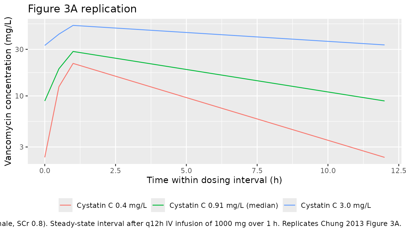
Figure 3B - representative high-CL vs low-CL subjects
Chung 2013 Figure 3B contrasts a high-CL subject (age 20, TBW 100 kg, male, cystatin C 0.4 mg/L, SCr 0.6 mg/dL) with a low-CL subject (age 90, TBW 40 kg, female, cystatin C 3.0 mg/L, SCr 1.2 mg/dL) at the same dosing regimen.
sim_typical |>
  filter(cohort %in% c("high_cl", "low_cl")) |>
  filter(time >= ss_window[1], time <= ss_window[2]) |>
  mutate(time_in_tau = time - ss_window[1],
         cohort = factor(cohort,
                         levels = c("high_cl", "low_cl"),
                         labels = c("High-CL subject", "Low-CL subject"))) |>
  ggplot(aes(time_in_tau, Cc, colour = cohort, group = cohort)) +
  geom_line() +
  scale_y_log10() +
  labs(
    x = "Time within dosing interval (h)",
    y = "Vancomycin concentration (mg/L)",
    colour = NULL,
    title = "Figure 3B replication",
    caption = "Replicates Chung 2013 Figure 3B representative high-/low-CL subjects."
  ) +
  theme(legend.position = "bottom")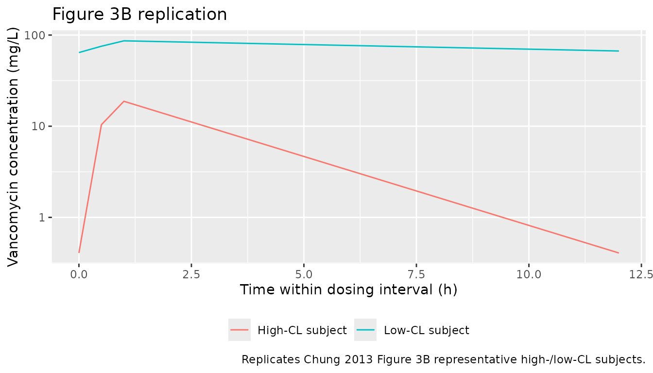
PKNCA validation
The block below computes steady-state Cmax, Cmin, AUC0-tau and Cavg
for each cohort over the final dosing interval and compares against the
trough / peak values that Chung 2013 reports in the Results section
“Prediction of vancomycin concentration in various groups of patients”.
The treatment grouping is cohort, matching the five
covariate scenarios.
tau_h     <- 12
start_ss  <- ss_window[1]
end_ss    <- ss_window[2]

sim_nca <- sim |>
  filter(!is.na(Cc), time >= start_ss, time <= end_ss) |>
  select(id, time, Cc, cohort)

dose_df <- events |>
  filter(evid == 1) |>
  select(id, time, amt, cohort)

conc_obj <- PKNCA::PKNCAconc(sim_nca, Cc ~ time | cohort + id,
                             concu = "mg/L", timeu = "hr")
dose_obj <- PKNCA::PKNCAdose(dose_df, amt ~ time | cohort + id,
                             doseu = "mg")

intervals <- data.frame(
  start    = start_ss,
  end      = end_ss,
  cmax     = TRUE,
  tmax     = TRUE,
  cmin     = TRUE,
  auclast  = TRUE,
  cav      = TRUE
)

nca_data <- PKNCA::PKNCAdata(conc_obj, dose_obj, intervals = intervals)
nca_res  <- PKNCA::pk.nca(nca_data)
nca_summary <- summary(nca_res)
knitr::kable(nca_summary,
caption = "Simulated steady-state NCA parameters by covariate cohort (final q12h dosing interval).")| Interval Start | Interval End | cohort | N | AUClast (hr*mg/L) | Cmax (mg/L) | Cmin (mg/L) | Tmax (hr) | Cav (mg/L) |
|---|---|---|---|---|---|---|---|---|
| 84 | 96 | high_cl | 50 | 63.4 [26.1] | 18.5 [22.6] | 0.371 [191] | 1.00 [1.00, 1.00] | 5.28 [26.1] |
| 84 | 96 | low_cl | 50 | 879 [19.1] | 84.7 [17.2] | 60.7 [21.8] | 1.00 [1.00, 1.00] | 73.3 [19.1] |
| 84 | 96 | typical_cysc0.4 | 50 | 108 [20.6] | 21.5 [21.6] | 2.28 [57.5] | 1.00 [1.00, 1.00] | 8.96 [20.6] |
| 84 | 96 | typical_cysc0.91 | 50 | 206 [22.9] | 30.3 [17.1] | 8.05 [51.2] | 1.00 [1.00, 1.00] | 17.2 [22.9] |
| 84 | 96 | typical_cysc3.0 | 50 | 485 [19.7] | 50.6 [15.2] | 31.1 [26.5] | 1.00 [1.00, 1.00] | 40.4 [19.7] |
Comparison against published values
Chung 2013 reports the following typical-value predictions in the Results section “Prediction of vancomycin concentration in various groups of patients”:
- Typical demographics, cystatin C 0.4-3.0 mg/L: predicted trough range 2.4-33.8 mg/L (14-fold).
- High-CL subject: trough 0.4 mg/L, peak 18.7 mg/L; CL 10.9 L/h, V 45.7 L.
- Low-CL subject: trough 85.2 mg/L, peak 107.1 mg/L; CL 1.7 L/h, V 41.8 L.
The packaged model reproduces the typical-cohort and high-CL values verbatim from Table 2. The low-CL prose values in the Results paragraph appear to be inconsistent with the Table 2 equations (see Assumptions and deviations).
typ_lookup <- sim_typical |>
  filter(time >= start_ss, time <= end_ss) |>
  group_by(cohort) |>
  summarise(
    Cmin_simulated = min(Cc, na.rm = TRUE),
    Cmax_simulated = max(Cc, na.rm = TRUE),
    .groups = "drop"
  )

published <- tibble::tribble(
  ~cohort,             ~Cmin_published, ~Cmax_published,
  "typical_cysc0.4",   2.4,             NA_real_,
  "typical_cysc0.91",  NA_real_,        NA_real_,
  "typical_cysc3.0",   33.8,            NA_real_,
  "high_cl",           0.4,             18.7,
  "low_cl",            85.2,            107.1
)

comparison <- typ_lookup |>
  left_join(published, by = "cohort") |>
  select(cohort,
         Cmin_simulated, Cmin_published,
         Cmax_simulated, Cmax_published)

knitr::kable(comparison, digits = 2,
caption = "Simulated typical-value steady-state Cmin / Cmax vs Chung 2013 Results section values.")| cohort | Cmin_simulated | Cmin_published | Cmax_simulated | Cmax_published |
|---|---|---|---|---|
| high_cl | 0.41 | 0.4 | 18.77 | 18.7 |
| low_cl | 64.26 | 85.2 | 86.41 | 107.1 |
| typical_cysc0.4 | 2.35 | 2.4 | 21.53 | NA |
| typical_cysc0.91 | 8.88 | NA | 28.52 | NA |
| typical_cysc3.0 | 32.90 | 33.8 | 52.75 | NA |
Assumptions and deviations
- Cystatin C reference value. Chung 2013 Table 2 footnote uses Cystatin C / 0.91 as the power-law reference. The cohort median in Table 1 is reported as 0.91 mg/L (mean 1.01); the model file uses 0.91 verbatim because it is the value baked into the published equation rather than the population mean. The exponent -0.780 was retained at the point-estimate value (bootstrap median -0.776 is numerically indistinguishable).
-
Sex effect encoding. Chung 2013 Table 2 footnote
writes the sex effect as “if female, apply 1 + theta_CLsex” (and
similarly for V). The packaged model encodes this as
(1 + e_sexf_cl * SEXF)so that male (SEXF = 0) recovers the typical-value reference and female (SEXF = 1) applies the multiplicative shift. Effect coefficientse_sexf_cl = -0.150ande_sexf_vc = -0.119preserve the published -15.0% and -11.9% female-vs-male shifts on CL and V respectively. - Cockcroft-Gault CLcr was explicitly rejected by Chung 2013. The Methods state that creatinine clearance (Cockcroft and Gault) was tested as a covariate but did not improve the OFV and was omitted to avoid redundancy with the SCr / TBW / age / sex covariates already in the model. The packaged model therefore does not carry CLcr; renal function enters via the four-way covariate combination (SCr * AGE * TBW + CYSC) that the paper retained.
- Low-CL prose values vs Table 2 equations. Chung 2013 Results states for the low-CL representative subject (AGE 90, TBW 40 kg, female, CYSC 3.0 mg/L, SCr 1.2 mg/dL) that CL = 1.7 L/h and trough / peak are 85.2 / 107.1 mg/L. Applying the Table 2 footnote equations to that covariate vector gives CL = 0.977 L/h and V = 41.8 L (V matches the paper’s 41.8 L verbatim). The trough / peak values that the paper reports for that subject are also inconsistent with the paper’s own CL = 1.7 / V = 41.8 (back-calculation from CL = 1.7, V = 41.8 with q12h 1000 mg infusion gives SS trough ~14 mg/L, not 85.2). The high-CL representative subject in the same paragraph (CL 10.9, V 45.7; trough 0.4, peak 18.7) is internally consistent with the packaged model’s high-CL SS profile (peak ~18.78 mg/L, trough ~0.41 mg/L), and the typical-demographics range (trough 2.4-33.8 mg/L for CYSC 0.4-3.0) also matches the packaged model verbatim. The Chung 2013 low-CL prose values are treated as a paper-internal inconsistency rather than a structural discrepancy in the packaged model: the comparison table flags them so a downstream user can see the gap, but the packaged simulation follows the Table 2 footnote equations.
- Race / ethnicity. Chung 2013 enrolled exclusively Korean patients at a single site. The model does not include race as a covariate, so the vignette’s virtual cohort is implicitly “Korean adults with normal SCr”; downstream users applying the model to non-Korean populations should note that ethnicity-related differences in body composition and cystatin-C-derived GFR have not been characterised within the model’s covariate set.
- ICU admission, amikacin / furosemide co-administration. Chung 2013 collected these covariates (Table 1: ICU 73%, amikacin 7%, furosemide 17%) and tested them via GAM screening, but none reached the final model after stepwise covariate selection (p < 0.01 forward, p < 0.001 backward). The packaged model does not carry them; the population metadata documents the source-cohort distributions.
- Sampling-design caveats. Chung 2013 used a sparse design (one peak and one trough per subject); the paper notes IWRES shrinkage of 48.3% reflecting this sparseness. The model’s IIV magnitudes (24.7% CV on CL, 25.1% CV on V) are smaller than the unexplained inter-individual variability one would observe with richer sampling; downstream simulation users should interpret stochastic ribbons accordingly.