Enteric-coated aspirin (Koh 2025)
Source:vignettes/articles/Koh_2025_aspirin.Rmd
Koh_2025_aspirin.RmdModel and source
- Citation: Koh JE, Khwarg J, Yu KS, Lee S, Jang IJ, Lee S. Population Pharmacokinetic and Pharmacodynamic Modeling of Enteric-Coated Aspirin Capsule and Tablet Formulations in Healthy Subjects. Drug Des Devel Ther. 2025;19:7853-7863. doi:10.2147/DDDT.S533428
- Description: Joint population PK-PD model for enteric-coated aspirin in healthy Korean adults (Koh 2025; two phase I studies, 100 mg once daily for 5 days). Parallel dual absorption – a zero-order arm with a lag time plus a first-order arm – delivers acetylsalicylic acid (ASA) into a pre-systemic compartment that drains by two competing first-order routes: intact ASA into the one-compartment ASA disposition, and gut-hydrolysed salicylic acid (SA) straight into the two-compartment SA disposition. Systemic ASA is eliminated entirely by conversion to SA (kmet), so apparent ASA clearance is kmet * V3/F = 69.8 L/h. Body weight enters kmet and SA clearance as power functions normalised to the 68.35 kg cohort median, and the enteric-coated capsule absorbs about four times faster than the enteric-coated tablet (ka 0.22 vs 0.053 1/h). A turnover model with an Imax function on ASA concentration inhibits serum thromboxane B2 production.
- Article: https://doi.org/10.2147/DDDT.S533428
- Supplement (Table S1 + Appendix 1, the complete Monolix model code): https://www.dovepress.com/article/supplementary_file/533428/533428%20Revised%20Supplemental%20Materials.pdf
Koh 2025 fits acetylsalicylic acid (ASA), its hydrolysis metabolite salicylic acid (SA), and serum thromboxane B2 (TXB2) simultaneously. The PK is a one-compartment ASA disposition plus a two-compartment SA disposition, fed by a parallel dual-absorption input and an explicit pre-systemic (gut) metabolism step. The PD is an indirect-response (turnover) model in which ASA inhibits TXB2 production through an Imax function.
Population
The model was built on pooled period-1 data from two open-label, two-period, one-sequence crossover phase I aspirin-rabeprazole interaction studies in healthy Korean volunteers (NCT05481307 and NCT05699070). Period 1 is aspirin alone – 100 mg once daily for 5 days – without the rabeprazole perpetrator.
44 subjects contributed 779 observations (317 ASA plasma, 379 SA plasma, 83 TXB2 serum): 21 received the enteric-coated capsule (Astrix, Boryungbio, Korea) and 23 the enteric-coated tablet (Aspirin Protect, Bayer, Germany). 41 were male and 3 female (6.8%). Median (min-max) age was 29 (20-49) years, height 174.55 (157.7-185.5) cm, weight 68.35 (55.6-89.5) kg and BMI 22.65 (19.5-26.9) kg/m2 (Koh 2025 Table S1). Enrolment required weight 50.0-90.0 kg and BMI 18.0-27.0 kg/m2, so the weight covariate is informed only over roughly 55-90 kg.
PK was sampled at 0, 0.5, 1, 1.5, 2, 2.5, 3, 3.5, 4, 5, 6, 7, 8, 12 and 24 h on days 1 and 5. TXB2 was sampled only pre-dose on day 1 and 24 h after the day-5 dose – 83 samples in total, which is why Imax, IC50 and the Hill coefficient had to be fixed. Estimation was by SAEM in Monolix 2021R1.
The same information is available programmatically via
readModelDb("Koh_2025_aspirin")()$population.
Source trace
Every ini() entry in
inst/modeldb/specificDrugs/Koh_2025_aspirin.R carries an
in-file comment naming its source. The table below collects them.
| Equation / parameter | Value | Source location |
|---|---|---|
| Dual absorption, pre-systemic split, ASA + SA ODEs | n/a | Koh 2025 Figure 1; Supplement Appendix 1 (Monolix code) |
| TXB2 turnover with Imax inhibition | n/a | Koh 2025 Figure 1 inset; Supplement Appendix 1 |
| Power covariate form, median-normalised | n/a | Koh 2025 Covariate Analysis, displayed equation |
| Logit-normal IIV on the zero-order fraction | n/a | Koh 2025 Model Development, displayed equation |
| Percent TXB2 inhibition | n/a | Koh 2025 Evaluation and Simulation, displayed equation |
logitfdepot (from fr = 0.69) |
0.31 | Table 1, fr, RSE 4.99% (complement; see Errata) |
lka_capsule |
0.22 1/h | Table 1, ka capsule, RSE 21.8% |
lka_tablet (fixed) |
0.053 1/h | Table 1, ka tablet, no RSE |
ld1 (Tk0) |
1.58 h | Table 1, RSE 15.8% |
ltlag (Lag0) |
2.81 h | Table 1, RSE 8.26% |
lk_presystemic_central (k23) |
2.32 1/h | Table 1, RSE 4.11% |
lk_presystemic_central_sa (k24, fixed) |
0.57 1/h | Table 1, no RSE; fixed from Koh 2025 ref 14 |
lkmet (k34) |
2.97 1/h | Table 1, RSE 11.7% |
e_wt_kmet |
1.31 | Table 1, beta weight_k34, RSE 30.9% |
lvc (V3/F) |
23.51 L | Table 1, RSE 12.3% |
lcl_sa (CLm/F) |
2.76 L/h | Table 1, RSE 3.86% |
e_wt_cl_sa |
1.42 | Table 1, beta weight_CLm, RSE 22.8% |
lvc_sa (V4/F) |
7.5 L | Table 1, RSE 2.6% |
lq_sa (Q/F, fixed) |
0.08 L/h | Table 1, no RSE; fixed from ref 14 |
lvp_sa (V5/F, fixed) |
1.98 L | Table 1, no RSE; fixed from ref 14 |
lrbase (R0) |
26.4 ug/L | Table 1, RSE 7.67% |
lkout |
0.023 1/h | Table 1, RSE 5.51% |
limax (fixed) |
1 | Table 1, no RSE |
lic50 (fixed) |
0.0036 umol/L | Table 1 numeral 0.0036 with the unit corrected from mol/L to umol/L; see Errata |
lhill (fixed) |
1 | Table 1, Gamma, no RSE |
| IIV variances (7) | SD^2 | Table 1 Random effects, footnote a (“standard deviations”) |
propSd, propSd_sa,
addSd_TXB2
|
0.41, 0.17, 2.58 | Table 1 Residual error |
| Weight median 68.35 kg | Table S1, Total column |
Structural identities
Two derived quantities the paper states in its Discussion are exact algebraic consequences of Table 1, so they are a free transcription check on the values that feed them.
ui <- rxode2::rxode(readModelDb("Koh_2025_aspirin"))
#> ℹ parameter labels from comments will be replaced by 'label()'
th <- ui$theta

cl_asa   <- exp(th[["lkmet"]]) * exp(th[["lvc"]])          # CL/F = k34 * V3/F
vss_sa   <- exp(th[["lvc_sa"]]) + exp(th[["lvp_sa"]])      # V4/F + V5/F

identities <- tibble::tibble(
  Quantity = c("ASA CL/F = k34 * V3/F (L/h)", "SA volume = V4/F + V5/F (L)"),
  Model    = c(cl_asa, vss_sa),
  Published = c(69.8, 9.48),
  Source   = c("Koh 2025 Discussion", "Koh 2025 Discussion")
)
knitr::kable(identities, digits = 2,
caption = "Derived quantities stated in the paper's Discussion.")| Quantity | Model | Published | Source |
|---|---|---|---|
| ASA CL/F = k34 * V3/F (L/h) | 69.82 | 69.80 | Koh 2025 Discussion |
| SA volume = V4/F + V5/F (L) | 9.48 | 9.48 | Koh 2025 Discussion |
Virtual cohort
Original observed data are not public. The simulations below use virtual cohorts at the published weight median (68.35 kg), which is the covariate reference, so the weight terms sit exactly at 1 and the comparison isolates the structural and PD parameters.
An rxode2 workaround is required
Through the rxUi interface, rxode2 5.1.7 fails to solve
this model when the modelled infusion duration
(dur(presystemic)) and the absorption lag
(alag(presystemic)) are both attached to the pre-systemic
compartment and a second compartment (depot, the
first-order arm) is dosed at an earlier time. It aborts with
Duration is zero/negative. The identical ODE system solves
correctly through plain rxode2::rxode2(), so this is an
interface-layer defect rather than a problem with the model.
The workaround used below is numerically identical: the modelled
duration is removed from the simulation copy of the model and the same
per-subject duration is supplied as an event-table dur
column instead. alag() – and therefore the inter-individual
variability on the lag time – is left in the model and still applies.
The between-subject variability on the zero-order duration is preserved
by drawing the random effects explicitly and computing each subject’s
d1. The packaged model file keeps the faithful
dur() / alag() encoding.
set.seed(20250822)

MW   <- 180.157      # g/mol, acetylsalicylic acid
NARM <- 200          # subjects per arm (cohort cap)

sim_ui <- suppressMessages(rxode2::model(ui, -dur(presystemic)))
om     <- ui$omega
enms   <- dimnames(om)[[1]]

# One eta matrix, reused by every arm (common random numbers). Pairing the arms
# subject-for-subject strips Monte Carlo noise out of the capsule-vs-tablet and
# 80-vs-160 mg contrasts, which are exactly the comparisons the paper draws, and
# it makes the dose-proportionality identity below exact rather than approximate.
ETAS <- as.data.frame(mvtnorm::rmvnorm(NARM, sigma = om))
names(ETAS) <- enms

draw_etas <- function(n, id_offset = 0L) {
  stopifnot(n == NARM)
  e <- ETAS
  e$id <- id_offset + seq_len(n)
  e
}

# One arm = one (dose, formulation) cell. `obs_times` lets a cheap cell reuse
# the machinery with only the four evaluation times the figure needs.
make_cohort <- function(n, dose_mg, cap, obs_times, dose_times,
                        id_offset = 0L, label = NULL) {
  etas <- draw_etas(n, id_offset)
  d1_i <- exp(th[["ld1"]] + etas$etald1)
  amt  <- dose_mg / MW * 1e3                       # mg -> umol (mg/(g/mol) = mmol)

  fo <- expand.grid(id = etas$id, time = dose_times)
  fo$amt <- amt; fo$cmt <- "depot"; fo$evid <- 1L
  fo$rate <- 0;  fo$dur <- 0;       fo$dvid <- NA_integer_

  zo <- expand.grid(id = etas$id, time = dose_times)
  zo$amt <- amt; zo$cmt <- "presystemic"; zo$evid <- 1L; zo$rate <- 0
  zo$dur <- d1_i[match(zo$id, etas$id)]; zo$dvid <- NA_integer_

  ob <- expand.grid(id = etas$id, time = obs_times)
  ob$amt <- NA_real_; ob$cmt <- NA_character_; ob$evid <- 0L
  ob$rate <- 0; ob$dur <- 0; ob$dvid <- 1L

  ev <- dplyr::arrange(rbind(fo, zo, ob), id, time, dplyr::desc(evid))
  ev <- dplyr::left_join(ev, etas, by = "id")
  ev$WT           <- 68.35
  ev$FORM_CAPSULE <- cap
  ev$formulation  <- ifelse(cap == 1, "Enteric-coated capsule", "Enteric-coated tablet")
  ev$dose_mg      <- dose_mg
  ev$arm          <- label %||% paste(ev$formulation, dose_mg, "mg")
  ev
}
`%||%` <- function(a, b) if (is.null(a)) b else a

solve_arm <- function(ev, model = sim_ui) {
  s <- rxode2::rxSolve(model, ev, omega = NA, useLinCmt = FALSE,
                       keep = c("formulation", "dose_mg", "arm", "WT"),
                       returnType = "data.frame")
  s[!duplicated(s[, c("id", "time")]), ]
}
Simulation: the 7-day external-validation scenario
Koh 2025 evaluated the final model against an external study in which 80 and 160 mg enteric-coated aspirin were given daily for 7 days (Figures 2 and 3). The four arms below reproduce that design: 2 doses x 2 formulations, 200 subjects each.
dose_times <- seq(0, 144, by = 24)                       # 7 daily doses
obs_times  <- sort(unique(c(seq(0, 24, by = 0.5),
                            seq(144, 168, by = 0.5),
                            seq(0, 168, by = 6))))

arms <- tibble::tribble(
  ~dose_mg, ~cap, ~offset,
  80,       1,    0L,
  160,      1,    1000L,
  80,       0,    2000L,
  160,      0,    3000L
)

events <- dplyr::bind_rows(lapply(seq_len(nrow(arms)), function(i) {
  make_cohort(NARM, arms$dose_mg[i], arms$cap[i],
              obs_times, dose_times, id_offset = arms$offset[i])
}))
stopifnot(!anyDuplicated(unique(events[, c("id", "time", "evid")])))

sim <- solve_arm(events)
#> Warning: multi-subject simulation without without 'omega'
Figure 2 – ASA and SA concentration-time profiles
Koh 2025 Figure 2 plots ASA and SA on a semi-log scale in nmol/L, overlaying the observed external data on the simulated 5th-95th percentile band. The replication below shows the same quantity for day 1 (panels A, B, E, F) and the day-7 dosing interval (panels C, D, G, H).
prof <- sim |>
  dplyr::select(id, time, Cc, Cc_sa, formulation, dose_mg) |>
  tidyr::pivot_longer(c(Cc, Cc_sa), names_to = "analyte", values_to = "conc") |>
  dplyr::mutate(
    analyte = dplyr::recode(analyte, Cc = "ASA", Cc_sa = "SA"),
    nmol_L  = conc * 1000,                    # umol/L -> nmol/L, the figure's unit
    window  = dplyr::case_when(time <= 24 ~ "Day 1 (0-24 h)",
                               time >= 144 ~ "Day 7 (144-168 h)",
                               TRUE ~ NA_character_)
  ) |>
  dplyr::filter(!is.na(window), nmol_L > 0)

prof |>
  dplyr::group_by(time, analyte, dose_mg, window) |>
  dplyr::summarise(Q05 = quantile(nmol_L, 0.05), Q50 = median(nmol_L),
                   Q95 = quantile(nmol_L, 0.95), .groups = "drop") |>
  ggplot(aes(time, Q50)) +
  geom_ribbon(aes(ymin = Q05, ymax = Q95), alpha = 0.2) +
  geom_line() +
  facet_grid(analyte ~ window + dose_mg, scales = "free_x") +
  scale_y_log10() +
  labs(x = "Time (h)", y = "Concentration (nmol/L)",
       title = "Figure 2 -- ASA and SA after 80 and 160 mg daily",
       caption = "Replicates Figure 2 of Koh 2025 (median and 5th-95th percentiles).")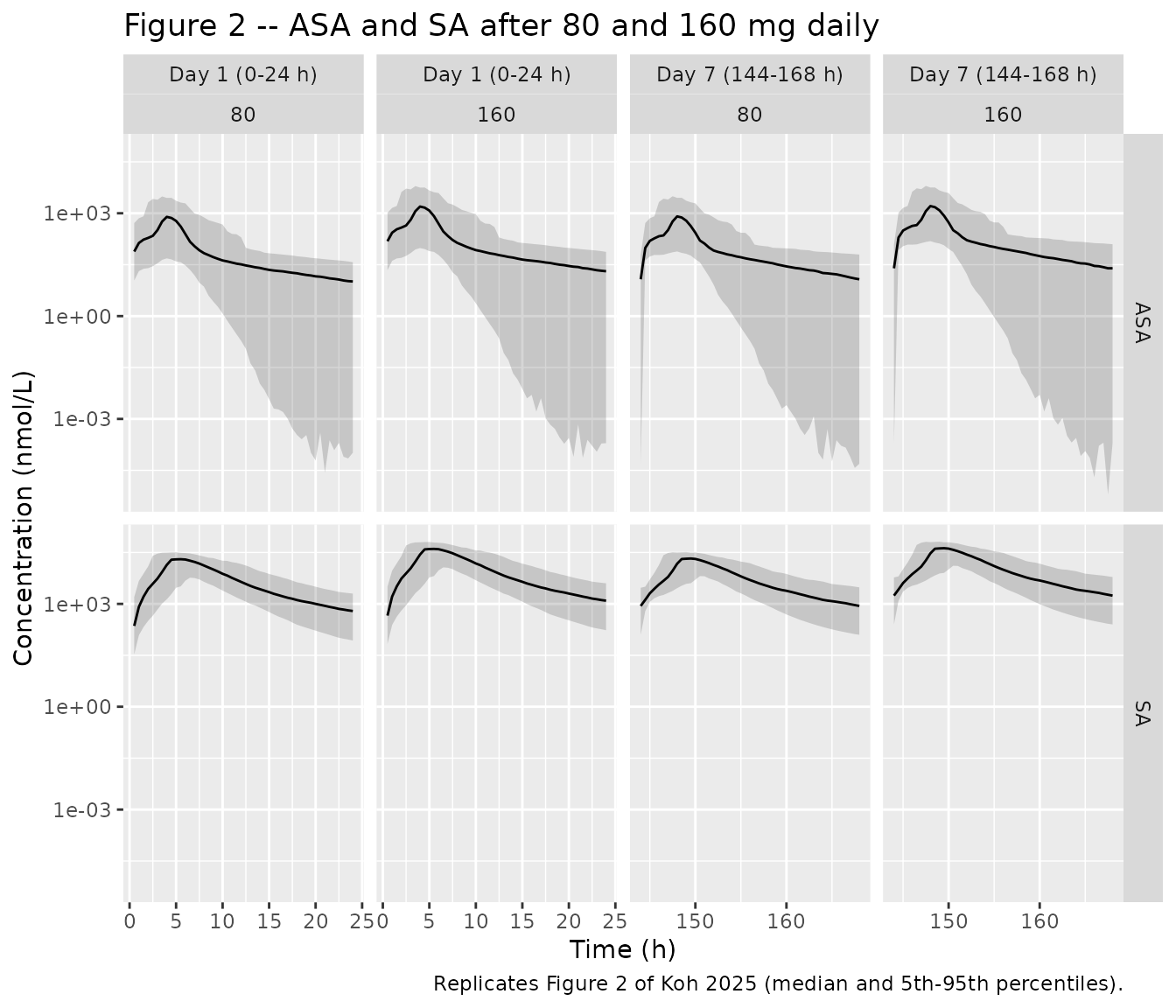
Figure 2’s y-axes are in nmol/L, which makes them a quantitative check on the concentration base of this implementation – one that is completely independent of the PD model. Reading the published median (solid) lines off panels A, B, E and F gives an ASA peak of roughly 700-1000 nmol/L at about 4 h after 80 mg and 15000-25000 nmol/L for SA at about 5-6 h, doubling at 160 mg. Day 1 of the 7-day regimen is a single dose for this purpose, since ASA does not accumulate.
peaks <- prof |>
  dplyr::filter(window == "Day 1 (0-24 h)", dose_mg %in% c(80, 160)) |>
  dplyr::group_by(analyte, dose_mg, time) |>
  dplyr::summarise(med = median(nmol_L), .groups = "drop_last") |>
  dplyr::slice_max(med, n = 1) |>
  dplyr::ungroup() |>
  dplyr::arrange(analyte, dose_mg)

peaks |>
  dplyr::rename("Analyte" = analyte, "Dose (mg)" = dose_mg,
                "Tmax of the median (h)" = time,
                "Median peak (nmol/L)" = med) |>
  knitr::kable(digits = c(0, 0, 2, 0),
caption = "Simulated day-1 median peak concentrations, against the Koh 2025 Figure 2 axes.")| Analyte | Dose (mg) | Tmax of the median (h) | Median peak (nmol/L) |
|---|---|---|---|
| ASA | 80 | 4.0 | 785 |
| ASA | 160 | 4.0 | 1570 |
| SA | 80 | 5.5 | 20085 |
| SA | 160 | 5.5 | 40170 |
pk_at <- function(a, d, col) peaks[[col]][peaks$analyte == a & peaks$dose_mg == d]

# 1. Peak heights land inside the windows read off the published Figure 2 axes.
stopifnot(dplyr::between(pk_at("ASA",  80, "med"),    400,  1500))
stopifnot(dplyr::between(pk_at("ASA", 160, "med"),    800,  3000))
stopifnot(dplyr::between(pk_at("SA",   80, "med"),  12000, 30000))
stopifnot(dplyr::between(pk_at("SA",  160, "med"),  25000, 60000))

# 2. Peaks occur when the figure says they do.
stopifnot(dplyr::between(pk_at("ASA", 80, "time"), 3, 6))
stopifnot(dplyr::between(pk_at("SA",  80, "time"), 4, 7))

# 3. The PK is linear in dose and the arms share random effects, so doubling the
#    dose must double the median profile EXACTLY. This is an identity, not a
#    tolerance: it fails if the dose conversion or the eta pairing is wrong.
for (a in c("ASA", "SA")) {
  stopifnot(abs(pk_at(a, 160, "med") / pk_at(a, 80, "med") - 2) < 1e-8)
}
The peak heights and times sit on the published curves, which fixes
the concentration base at umol/L (the model’s internal unit) and
therefore fixes the scale against which the IC50 unit
correction in the Errata is judged.
Figure 3 – TXB2 inhibition
Figure 3D of Koh 2025 prints twelve simulated percent-inhibition
values, one per (formulation, dose, time) cell at 24, 144 and 168 h.
That panel is the tightest answer key the paper offers, so it is used
here as a quantitative gate. Percent inhibition follows the paper’s own
definition,
(TXB2_baseline - TXB2_postdose) / TXB2_baseline * 100,
computed per subject against that subject’s own pre-dose baseline and
then summarised by the median.
pct_inhibition <- function(s, times = c(24, 144, 168)) {
  base <- s |> dplyr::filter(time == 0) |> dplyr::select(id, base = TXB2)
  s |>
    dplyr::filter(time %in% times) |>
    dplyr::inner_join(base, by = "id") |>
    dplyr::mutate(pct = (base - TXB2) / base * 100)
}

inh <- pct_inhibition(sim) |>
  dplyr::group_by(formulation, dose_mg, time) |>
  dplyr::summarise(simulated = median(pct), .groups = "drop")

published_3d <- tibble::tribble(
  ~formulation,             ~dose_mg, ~time, ~published,
  "Enteric-coated capsule", 80,       24,    37.03,
  "Enteric-coated capsule", 80,       144,   83.57,
  "Enteric-coated capsule", 80,       168,   84.87,
  "Enteric-coated capsule", 160,      24,    38.28,
  "Enteric-coated capsule", 160,      144,   86.39,
  "Enteric-coated capsule", 160,      168,   87.74,
  "Enteric-coated tablet",  80,       24,    39.51,
  "Enteric-coated tablet",  80,       144,   89.14,
  "Enteric-coated tablet",  80,       168,   90.53,
  "Enteric-coated tablet",  160,      24,    39.77,
  "Enteric-coated tablet",  160,      144,   89.72,
  "Enteric-coated tablet",  160,      168,   91.11
)

cmp3d <- dplyr::inner_join(inh, published_3d,
                           by = c("formulation", "dose_mg", "time")) |>
  dplyr::mutate(difference = simulated - published)

cmp3d |>
  dplyr::rename("Formulation" = formulation, "Dose (mg)" = dose_mg,
                "Time (h)" = time, "Simulated (%)" = simulated,
                "Koh 2025 Figure 3D (%)" = published,
                "Difference (pp)" = difference) |>
  knitr::kable(digits = 2,
caption = "Simulated vs published median TXB2 inhibition, all twelve Figure 3D cells.")| Formulation | Dose (mg) | Time (h) | Simulated (%) | Koh 2025 Figure 3D (%) | Difference (pp) |
|---|---|---|---|---|---|
| Enteric-coated capsule | 80 | 24 | 32.67 | 37.03 | -4.36 |
| Enteric-coated capsule | 80 | 144 | 74.56 | 83.57 | -9.01 |
| Enteric-coated capsule | 80 | 168 | 75.76 | 84.87 | -9.11 |
| Enteric-coated capsule | 160 | 24 | 35.78 | 38.28 | -2.50 |
| Enteric-coated capsule | 160 | 144 | 81.40 | 86.39 | -4.99 |
| Enteric-coated capsule | 160 | 168 | 82.70 | 87.74 | -5.04 |
| Enteric-coated tablet | 80 | 24 | 37.83 | 39.51 | -1.68 |
| Enteric-coated tablet | 80 | 144 | 89.79 | 89.14 | 0.65 |
| Enteric-coated tablet | 80 | 168 | 91.34 | 90.53 | 0.81 |
| Enteric-coated tablet | 160 | 24 | 39.90 | 39.77 | 0.13 |
| Enteric-coated tablet | 160 | 144 | 92.90 | 89.72 | 3.18 |
| Enteric-coated tablet | 160 | 168 | 94.47 | 91.11 | 3.36 |
The mean absolute error across all twelve published cells is 3.73 percentage points.
Figure 3C reports the same simulation pooled across the two formulations, and it is the panel behind the paper’s headline claim that steady-state inhibition “exceed[s] 80%” at both doses. It is scored separately below, because the claim is about the pooled quantity rather than about any single formulation arm.
inh_pooled <- pct_inhibition(sim) |>
  dplyr::group_by(dose_mg, time) |>
  dplyr::summarise(simulated = median(pct), .groups = "drop")

published_3c <- tibble::tribble(
  ~dose_mg, ~time, ~published,
  80,       24,    38.20,
  80,       144,   86.21,
  80,       168,   87.56,
  160,      24,    38.99,
  160,      144,   87.97,
  160,      168,   89.34
)

cmp3c <- dplyr::inner_join(inh_pooled, published_3c, by = c("dose_mg", "time")) |>
  dplyr::mutate(difference = simulated - published)

cmp3c |>
  dplyr::rename("Dose (mg)" = dose_mg, "Time (h)" = time,
                "Simulated (%)" = simulated,
                "Koh 2025 Figure 3C (%)" = published,
                "Difference (pp)" = difference) |>
  knitr::kable(digits = 2,
caption = "Simulated vs published formulation-pooled TXB2 inhibition (Figure 3C).")| Dose (mg) | Time (h) | Simulated (%) | Koh 2025 Figure 3C (%) | Difference (pp) |
|---|---|---|---|---|
| 80 | 24 | 36.60 | 38.20 | -1.60 |
| 80 | 144 | 86.21 | 86.21 | 0.00 |
| 80 | 168 | 87.60 | 87.56 | 0.04 |
| 160 | 24 | 39.15 | 38.99 | 0.16 |
| 160 | 144 | 90.82 | 87.97 | 2.85 |
| 160 | 168 | 92.30 | 89.34 | 2.96 |
# The model must reproduce the paper's stated conclusions, not merely land in
# the right decade.
ss  <- cmp3d |> dplyr::filter(time == 168)
ss_pooled <- cmp3c |> dplyr::filter(time == 168)

# 1. The paper's headline PD claim, scored on the quantity the paper actually
#    claims it of: the formulation-pooled steady-state inhibition (Figure 3C)
#    exceeds the 80% adequacy criterion at both doses.
stopifnot(all(ss_pooled$simulated > 80))

# 2. The capsule gives slightly LOWER inhibition than the tablet at both doses
#    (Koh 2025 Results: "the enteric-coated capsule showed slightly lower TXB2
#    inhibition compared to the tablet formulation").
for (d in c(80, 160)) {
  cap_v <- ss$simulated[ss$dose_mg == d & ss$formulation == "Enteric-coated capsule"]
  tab_v <- ss$simulated[ss$dose_mg == d & ss$formulation == "Enteric-coated tablet"]
  stopifnot(cap_v < tab_v)
}

# 3. Inhibition rises with dose within each formulation (Figure 3D).
for (fm in unique(ss$formulation)) {
  stopifnot(ss$simulated[ss$formulation == fm & ss$dose_mg == 160] >
            ss$simulated[ss$formulation == fm & ss$dose_mg ==  80])
}

# 4. Inhibition accumulates over the week: 24 h well below steady state.
stopifnot(all(cmp3d$simulated[cmp3d$time == 24] < 55))
stopifnot(all(cmp3d$simulated[cmp3d$time == 168] >
              cmp3d$simulated[cmp3d$time == 24]))

# 5. Quantitative agreement with the published bars. The tablet arms track the
#    paper closely; the capsule arms are the residual deviation documented in
#    the Errata, so the bound is set by the worst cell rather than by the mean.
stopifnot(mae_3d < 5)
stopifnot(mean(abs(cmp3c$difference)) < 5)
stopifnot(max(abs(cmp3d$difference)) < 12)
cmp3d |>
  tidyr::pivot_longer(c(simulated, published), names_to = "source",
                      values_to = "pct") |>
  dplyr::mutate(source = dplyr::recode(source, simulated = "This implementation",
                                       published = "Koh 2025 Figure 3D")) |>
  ggplot(aes(factor(time), pct, fill = source)) +
  geom_col(position = position_dodge(width = 0.8), width = 0.75) +
  facet_grid(dose_mg ~ formulation) +
  labs(x = "Time (h)", y = "Inhibition of thromboxane B2 (%)", fill = NULL,
       title = "Figure 3D -- simulated vs published TXB2 inhibition",
       caption = "Replicates Figure 3D of Koh 2025.") +
  theme(legend.position = "top")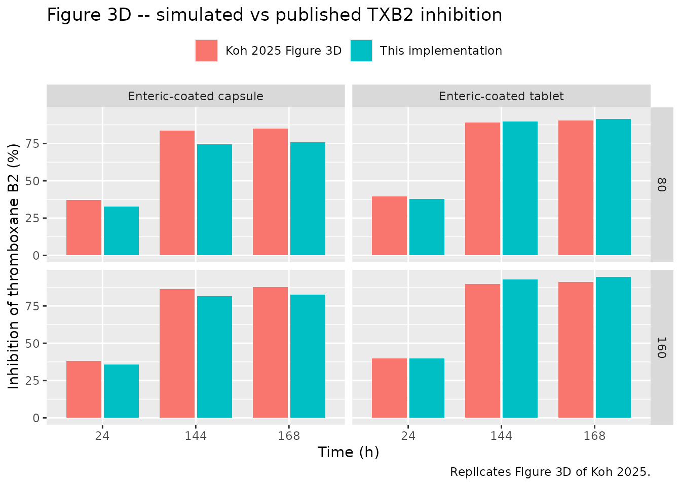
The TXB2 concentration-time profiles of Figure 3A and 3B fall out of the same simulation.
sim |>
  dplyr::group_by(time, formulation, dose_mg) |>
  dplyr::summarise(Q05 = quantile(TXB2, 0.05), Q25 = quantile(TXB2, 0.25),
                   Q50 = median(TXB2), Q75 = quantile(TXB2, 0.75),
                   Q95 = quantile(TXB2, 0.95), .groups = "drop") |>
  ggplot(aes(time, Q50)) +
  geom_ribbon(aes(ymin = Q05, ymax = Q95), alpha = 0.15) +
  geom_ribbon(aes(ymin = Q25, ymax = Q75), alpha = 0.25) +
  geom_line() +
  facet_grid(dose_mg ~ formulation) +
  scale_x_continuous(breaks = seq(0, 168, by = 24)) +
  labs(x = "Time (h)", y = "Serum TXB2 (ug/L)",
       title = "Figure 3A / 3B -- serum TXB2 over 7 days of daily dosing",
       caption = "Replicates Figures 3A and 3B of Koh 2025.")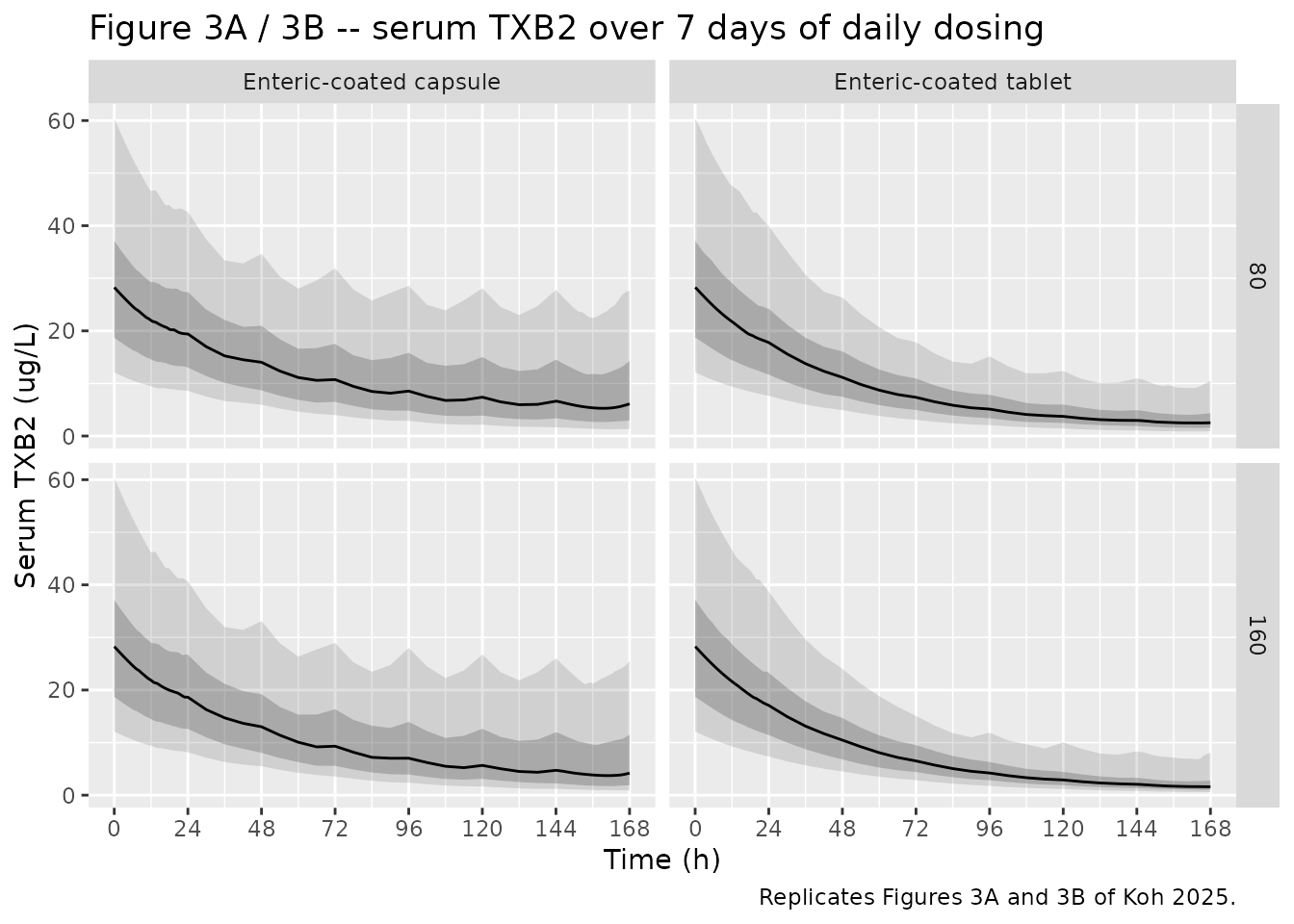
PKNCA validation
The paper does not publish an NCA table, but this model has two exact mass-balance identities that make far stricter tests than a median comparison:
-
ASA. Systemic ASA is eliminated only by conversion
to SA, and only the fraction
k23 / (k23 + k24)of the dose reaches the ASA central compartment at all. SoAUCinf_ASA = Dose * k23 / (k23 + k24) / (kmet * vc)per subject. -
SA. Both pre-systemic hydrolysis and systemic
conversion terminate in SA, and SA’s only exit is
CLm/F. Every absorbed micromole therefore passes through SA, givingAUCinf_SA = Dose / cl_saper subject – independent of every absorption and distribution parameter.
A single 100 mg dose (the dose the model was built on) is simulated for the NCA.
nca_obs <- sort(unique(c(seq(0, 12, by = 0.25), seq(12, 48, by = 1),
                         seq(48, 168, by = 4))))
nca_events <- dplyr::bind_rows(
  make_cohort(NARM, 100, 1, nca_obs, dose_times = 0, id_offset = 0L),
  make_cohort(NARM, 100, 0, nca_obs, dose_times = 0, id_offset = 1000L)
)
stopifnot(!anyDuplicated(unique(nca_events[, c("id", "time", "evid")])))
nca_sim <- solve_arm(nca_events)
#> Warning: multi-subject simulation without without 'omega'
run_nca <- function(sim_df, conc_col) {
  d <- sim_df |>
    dplyr::mutate(Cc = .data[[conc_col]]) |>
    dplyr::filter(!is.na(Cc)) |>
    dplyr::select(id, time, Cc, formulation)
  d <- dplyr::bind_rows(
    d,
    d |> dplyr::distinct(id, formulation) |> dplyr::mutate(time = 0, Cc = 0)
  ) |>
    dplyr::distinct(id, formulation, time, .keep_all = TRUE) |>
    dplyr::arrange(id, formulation, time)

  dose_df <- nca_events |>
    dplyr::filter(evid == 1, cmt == "depot") |>
    dplyr::select(id, time, amt, formulation)

  intervals <- data.frame(start = 0, end = Inf, cmax = TRUE, tmax = TRUE,
                          aucinf.obs = TRUE, half.life = TRUE)
  suppressWarnings(PKNCA::pk.nca(PKNCA::PKNCAdata(
    PKNCA::PKNCAconc(d, Cc ~ time | formulation + id),
    PKNCA::PKNCAdose(dose_df, amt ~ time | formulation + id),
    intervals = intervals
  )))
}

nca_asa <- run_nca(nca_sim, "Cc")
nca_sa  <- run_nca(nca_sim, "Cc_sa")
# Per-subject expected AUCinf from the structural identities above.
ind <- nca_sim |>
  dplyr::distinct(id, formulation, kmet, vc, cl_sa,
                  k_presystemic_central, k_presystemic_central_sa)
dose_umol <- 100 / MW * 1e3
frac_asa  <- ind$k_presystemic_central /
  (ind$k_presystemic_central + ind$k_presystemic_central_sa)
ind$expected_asa <- dose_umol * frac_asa / (ind$kmet * ind$vc)
ind$expected_sa  <- dose_umol / ind$cl_sa

auc_of <- function(res) {
  as.data.frame(res) |>
    dplyr::filter(PPTESTCD == "aucinf.obs") |>
    dplyr::select(id, formulation, auc = PPORRES) |>
    dplyr::mutate(id = as.integer(as.character(id)))
}

chk <- ind |>
  dplyr::left_join(auc_of(nca_asa) |> dplyr::rename(auc_asa = auc),
                   by = c("id", "formulation")) |>
  dplyr::left_join(auc_of(nca_sa) |> dplyr::rename(auc_sa = auc),
                   by = c("id", "formulation")) |>
  dplyr::mutate(rel_asa = auc_asa / expected_asa,
                rel_sa  = auc_sa  / expected_sa)

id_tbl <- tibble::tibble(
  Identity = c("AUCinf ASA vs Dose * k23/(k23+k24) / (kmet * vc)",
               "AUCinf SA vs Dose / cl_sa"),
  `Median ratio`  = c(median(chk$rel_asa, na.rm = TRUE),
                      median(chk$rel_sa,  na.rm = TRUE)),
  `Min ratio`     = c(min(chk$rel_asa, na.rm = TRUE),
                      min(chk$rel_sa,  na.rm = TRUE)),
  `Max ratio`     = c(max(chk$rel_asa, na.rm = TRUE),
                      max(chk$rel_sa,  na.rm = TRUE))
)
knitr::kable(id_tbl, digits = 4,
caption = "Per-subject mass-balance identities. A correct implementation returns 1.")| Identity | Median ratio | Min ratio | Max ratio |
|---|---|---|---|
| AUCinf ASA vs Dose * k23/(k23+k24) / (kmet * vc) | 0.9970 | 0.9823 | 1.0101 |
| AUCinf SA vs Dose / cl_sa | 0.9998 | 0.9904 | 1.0003 |
# NCA extrapolates a finite tail, so allow a small deficit but no excess.
stopifnot(all(abs(chk$rel_sa  - 1) < 0.05, na.rm = TRUE))
stopifnot(all(abs(chk$rel_asa - 1) < 0.10, na.rm = TRUE))
nca_summary <- dplyr::bind_rows(
  as.data.frame(nca_asa) |> dplyr::mutate(Analyte = "ASA"),
  as.data.frame(nca_sa)  |> dplyr::mutate(Analyte = "SA")
) |>
  dplyr::filter(PPTESTCD %in% c("cmax", "tmax", "aucinf.obs", "half.life")) |>
  dplyr::group_by(Analyte, formulation, PPTESTCD) |>
  dplyr::summarise(median = median(PPORRES, na.rm = TRUE), .groups = "drop") |>
  tidyr::pivot_wider(names_from = PPTESTCD, values_from = median) |>
  dplyr::rename("Formulation" = formulation, "Cmax (umol/L)" = cmax,
                "Tmax (h)" = tmax, "AUC0-inf (umol*h/L)" = aucinf.obs,
                "t1/2 (h)" = half.life)

knitr::kable(nca_summary, digits = 2,
caption = "Simulated single-dose 100 mg NCA (median across 200 subjects per arm).")| Analyte | Formulation | AUC0-inf (umol*h/L) | Cmax (umol/L) | t1/2 (h) | Tmax (h) |
|---|---|---|---|---|---|
| ASA | Enteric-coated capsule | 6.16 | 2.78 | 3.98 | 4.25 |
| ASA | Enteric-coated tablet | 6.33 | 2.76 | 12.80 | 4.50 |
| SA | Enteric-coated capsule | 202.39 | 35.94 | 17.60 | 5.25 |
| SA | Enteric-coated tablet | 202.40 | 33.37 | 17.57 | 5.25 |
The capsule and tablet Tmax values differ in the direction the paper
reports: the capsule’s four-fold larger ka (0.22 vs 0.053
1/h) produces the earlier peak, and the tablet’s slow first-order arm
sustains ASA exposure for longer, which is exactly why the tablet
achieves marginally greater TXB2 inhibition despite identical
bioavailability.
Assumptions and deviations
-
Errata – Table 1’s IC50 unit is wrong by a factor of 1e6. Table 1 prints
IC50 (mol/L) 0.0036. Read literally that is 3.6 mmol/L, some three thousand times the model’s own peak ASA concentration, and the model then predicts essentially no TXB2 inhibition at all – contradicting the abstract (“exceeding 80%”), the Conclusion, and Figure 3. The correct unit is umol/L: the “u” was dropped. The printed numeral 0.0036 is preserved exactly; only the unit is corrected, and it is already in the model file’s umol/L base.The argument has two independent legs. The first fixes the concentration base without reference to the PD model at all: Figure 2’s axes are in nmol/L, and the simulated ASA and SA medians land on the published curves in both height and time (asserted in the Figure 2 section above). The second, with that base fixed, sweeps IC50 across the candidate unit readings and scores each against the twelve published Figure 3D bars. The sweep is recomputed here rather than quoted, so the table cannot drift from the model file:
sweep_grid <- tibble::tibble(
  reading  = c("nmol/L", "umol/L (adopted)", "mmol/L", "mol/L (as printed)"),
  umol_L   = c(0.0036e-3, 0.0036, 3.6, 3600)
)

# The sweep only ever reads the four scored times, so it re-solves a lean event
# table rather than the dense one used for the profile plots.
sweep_events <- dplyr::bind_rows(lapply(seq_len(nrow(arms)), function(i) {
  make_cohort(NARM, arms$dose_mg[i], arms$cap[i],
              obs_times = c(0, 24, 144, 168), dose_times = dose_times,
              id_offset = arms$offset[i])
}))

score_ic50 <- function(ic50_umol) {
  s <- rxode2::rxSolve(sim_ui, sweep_events, params = c(lic50 = log(ic50_umol)),
                       omega = NA, returnType = "data.frame",
                       keep = c("formulation", "dose_mg"))
  s <- s[!duplicated(s[, c("id", "time")]), ]
  cmp <- pct_inhibition(s) |>
    dplyr::group_by(formulation, dose_mg, time) |>
    dplyr::summarise(simulated = median(pct), .groups = "drop") |>
    dplyr::inner_join(published_3d, by = c("formulation", "dose_mg", "time"))
  ss <- cmp |> dplyr::filter(time == 168)
  tibble::tibble(
    mae   = mean(abs(cmp$simulated - cmp$published)),
    range = max(ss$simulated) - min(ss$simulated)
  )
}

sweep <- sweep_grid |>
  dplyr::bind_cols(dplyr::bind_rows(lapply(sweep_grid$umol_L, score_ic50)))
#> Warning: multi-subject simulation without without 'omega'
#> Warning: multi-subject simulation without without 'omega'
#> Warning: multi-subject simulation without without 'omega'
#> Warning: multi-subject simulation without without 'omega'

sweep |>
  dplyr::mutate(umol_L = formatC(umol_L, format = "g", digits = 3)) |>
  dplyr::rename("IC50 unit reading" = reading, "Value in umol/L" = umol_L,
                "MAE vs Figure 3D (pp)" = mae,
                "Spread across the 4 arms at 168 h (pp)" = range) |>
  knitr::kable(digits = 2, align = "lrrr",
caption = "Scoring each candidate reading of Table 1's IC50 unit against the twelve published Figure 3D bars.")| IC50 unit reading | Value in umol/L | MAE vs Figure 3D (pp) | Spread across the 4 arms at 168 h (pp) |
|---|---|---|---|
| nmol/L | 3.6e-06 | 7.40 | 0.04 |
| umol/L (adopted) | 0.0036 | 3.73 | 18.71 |
| mmol/L | 3.6 | 67.41 | 2.86 |
| mol/L (as printed) | 3.6e+03 | 71.47 | 0.00 |
adopted <- which(sweep$reading == "umol/L (adopted)")
potent  <- which(sweep$reading == "nmol/L")

# 1. The adopted reading is the best of the four, and by a wide margin.
stopifnot(which.min(sweep$mae) == adopted)
stopifnot(min(sweep$mae[-adopted]) > 1.5 * sweep$mae[adopted])

# 2. The minimum is interior: both neighbours in the candidate set are worse.
stopifnot(sweep$mae[adopted] < sweep$mae[adopted - 1])
stopifnot(sweep$mae[adopted] < sweep$mae[adopted + 1])

# 3. Figure 3D spreads 6.24 pp across its four arms at 168 h (91.11 - 84.87),
#    so the formulation and dose differences are a real feature of the published
#    simulation. A reading one decade more potent drives every arm to near-
#    complete inhibition and collapses that spread to nothing; the adopted
#    reading keeps it. This is the qualitative leg of the argument.
stopifnot(sweep$range[potent] < 1)
stopifnot(sweep$range[adopted] > 3)
The minimum is interior rather than at an edge of the candidate set, and it is the only reading that also preserves the paper’s qualitative result. A reading one decade more potent drives every arm to near-complete inhibition and erases the capsule-versus-tablet and 80-versus-160 mg differences that are the paper’s central findings; readings a decade or more weaker collapse inhibition altogether.
Note that this IC50 is not an in-vitro potency constant. It is the
fixed inhibition constant of a turnover model in which aspirin acts
irreversibly on circulating platelets, and a very low apparent value is
what that structure produces. Koh 2025 attributes it to reference 19
(Kimura 2014, doi:10.1177/1076029613488934); that article was not
available when this model was built, so the correction rests on the two
legs above rather than on the cited source. * Errata – the
capsule arms are under-predicted by roughly 5-9 percentage
points. With every parameter taken verbatim from Table 1, the
tablet arms reproduce Figure 3D closely (within about 3 pp) but the
capsule arms fall short, most visibly at 80 mg. This implementation
therefore exaggerates the capsule-versus-tablet gap relative to the
published simulation while preserving its direction. The formulation
enters only through ka, which acts on the first-order arm
carrying just 1 - fr = 31% of the dose, so the published gap is the more
surprising of the two; the likely cause is a difference between Simulx’s
and rxode2’s handling of the parallel zero-order plus first-order input
rather than a transcription error, but the paper does not publish enough
detail to settle it. No parameter was tuned to close the gap. *
Errata – the Discussion’s per-formulation steady-state values
are internally inconsistent with Figure 3D. The Discussion
states 87.7% (capsule) and 89.3% (tablet) at 160 mg, and 84.9% (capsule)
and 91.1% (tablet) at 80 mg. Only three of those four are Figure 3D
values: 87.74 is capsule/160, 84.87 is capsule/80 and 91.11 is
tablet/160 (not tablet/80, which is 90.53), while 89.3
matches the formulation-pooled Figure 3C value for 160 mg rather than
any tablet cell. Figure 3D, which labels every cell explicitly, is used
as the answer key here. * The zero-order absorbed fraction is
stored as its complement. Koh 2025 reports fr =
0.69 as the fraction absorbed by the zero-order arm.
The library canonical fdepot is the fraction absorbed via
the depot, i.e. the first-order arm, so the model file
stores logitfdepot = logit(1 - 0.69) and the zero-order arm
takes 1 - fdepot. Because
logit(1 - p) = -logit(p), the logit-normal IIV variance
carries over unchanged. * IIV variances are the published
standard deviations squared. Table 1’s footnote a states that
random effects are presented as standard deviations, so every
ini() variance is the tabulated omega squared. * An
rxode2 5.1.7 defect required a simulation-only workaround, as
described under “Virtual cohort” above. The packaged model file keeps
the faithful dur(presystemic) /
alag(presystemic) encoding; only the vignette’s simulation
copy moves the duration into the event table, where it is set to each
subject’s own d1, so the zero-order arm is unchanged. Two
checks in this vignette confirm the substitution behaves as intended
rather than silently dropping the input: the per-subject SA mass-balance
identity (AUCinf_SA = Dose / cl_sa) verifies that the full
dose is still delivered, and the Figure 2 timing assertions verify the
lag and duration still act – Lag0 = 2.81 h plus
Tk0 = 1.58 h puts the end of the zero-order input at 4.39
h, and the simulated ASA median peaks at 4 h. * Weight is held
at the 68.35 kg published median in all simulations, so the
weight terms on kmet and cl_sa evaluate to
exactly 1. The paper’s own Figure 2 and Figure 3 simulations are
likewise typical-weight predictions. * No race or sex
covariates. The study population is Korean and 93% male;
neither sex nor race was tested as a covariate, so neither appears in
the model. * Age, height and BMI were screened but not
retained by the paper’s stepwise covariate procedure. They are
recorded in the model’s covariatesDataExcluded metadata
rather than covariateData, since they are documentation
only. * The 24 h Figure 3D cells are the weakest
agreement. The paper’s own PD dataset contains TXB2 only at
pre-dose day 1 and 24 h after the day-5 dose, so the early part of the
inhibition time course is barely informed by data; the paper flags this
as a limitation.