Rifampicin (Clewe 2015)
Source:vignettes/articles/Clewe_2015_rifampicin.Rmd
Clewe_2015_rifampicin.RmdModel and source
- Citation: Clewe O., Goutelle S., Conte J. E. Jr., Simonsson U. S. H. (2015). A pharmacometric pulmonary model predicting the extent and rate of distribution from plasma to epithelial lining fluid and alveolar cells – using rifampicin as an example. European Journal of Clinical Pharmacology 71(3):313-319. doi:10.1007/s00228-014-1798-3. PK structure (one-compartment + single transit + enzyme-pool autoinduction) and the fixed autoinduction parameters (MTT, N, EMAX, EC50, kENZ) are inherited from Smythe et al. (2012) Antimicrob Agents Chemother 56(4):2091-2098 doi:10.1128/AAC.05792-11; see modellib(‘Svensson_2016_rifampicin’) for the same PK backbone applied to a TB sputum dataset.
- Description: Pharmacometric pulmonary distribution model for rifampicin in adults without tuberculosis: a one-compartment plasma PK model with single-transit oral absorption coupled to a Smythe 2012 enzyme-pool autoinduction structure (MTT, N, EMAX, EC50, kENZ all fixed from the upstream Smythe 2012 model) plus two effect compartments capturing distribution from plasma to epithelial lining fluid (ELF) and alveolar cells (AC); CL/F and Vc/F are FFM-allometrically scaled to 70 kg, the ELF and AC equilibration rate constants kELF and kAC are fixed to an equivalent 1-min half-life (instantaneous distribution at the single 4-h post-dose BAL sampling time), and only the unbound steady-state ELF/plasma and AC/plasma concentration ratios are estimated (1.28 and 5.5 after correction for the 20% rifampicin plasma free fraction).
- Article: https://doi.org/10.1007/s00228-014-1798-3
Population
The model was fit to 40 adult subjects without active tuberculosis (Clewe 2015 Methods, “Data” paragraph 1):
- 10 women without AIDS
- 10 men without AIDS
- 10 women with AIDS
- 10 men with AIDS
Subjects received rifampicin 600 mg orally once daily for 5 days; on day 5, plasma was sampled at approximately 2 h and 4 h post-dose (76 samples total across the cohort), and a single bronchoalveolar lavage (BAL) was performed at approximately 4 h after the last dose (32 ELF samples and 36 AC samples). The dataset was originally generated by Conte et al. (2004) and reused in Clewe 2015. Individual demographics (age, weight, height) are not tabulated in Clewe 2015 itself; the underlying Conte 2004 cohort is described as adult US subjects, and the analysis used HIV/AIDS status as a stratification variable but did NOT test it as a covariate on the PK (Clewe 2015 Discussion paragraph 5: “The influence of potential subpopulation-specific properties or covariates were not explored in this analysis”).
readModelDb("Clewe_2015_rifampicin")()$population
returns this metadata programmatically.
Source trace
Per-parameter origins are recorded next to each ini()
entry in
inst/modeldb/specificDrugs/Clewe_2015_rifampicin.R. The
table below collects them in one place for review.
| Element | Value | Source location |
|---|---|---|
lcl (CL/F) |
log(3.85 L/h) | Clewe 2015 Table 1, TV(CL/F)STD = 3.85 L/h (95% CI 2.26-8.68; RSE 3.1%) |
lvc (Vc/F) |
log(76.6 L) | Clewe 2015 Table 1, TV(Vc/F)STD = 76.6 L (95% CI 60.85-88.83; RSE 2.7%) |
lmtt (MTT) |
fixed(log(0.71 h)) | Clewe 2015 Table 1, MTT = 0.71 h FIX (carried from Smythe 2012) |
nn_fix (N) |
fixed(1) | Clewe 2015 Table 1, N = 1 FIX (carried from Smythe 2012) |
lemax (EMAX) |
fixed(log(1.04)) | Clewe 2015 Table 1, EMAX = 1.04 FIX (carried from Smythe 2012) |
lec50 (EC50) |
fixed(log(0.0705 mg/L)) | Clewe 2015 Table 1, EC50 = 0.0705 mg/L FIX (carried from Smythe 2012) |
lkenz (kENZ) |
fixed(log(0.0036 /h)) | Clewe 2015 Table 1, kENZ = 0.0036/h FIX (carried from Smythe 2012) |
lkelf (kELF) |
fixed(log(41.58 /h)) | Clewe 2015 Table 1, kELF = 41.58/h FIX (~1-min equilibration half-life) |
lkac (kAC) |
fixed(log(41.58 /h)) | Clewe 2015 Table 1, kAC = 41.58/h FIX (~1-min equilibration half-life) |
lrelf (R_ELF/plasma) |
log(0.26) | Clewe 2015 Table 1, R_ELF/plasma = 0.26 (95% CI 0.21-0.31; RSE 4.3%) |
lrac (R_AC/plasma) |
log(1.1) | Clewe 2015 Table 1, R_AC/plasma = 1.1 (95% CI 0.92-1.35; RSE 6.2%) |
lfdepot (F) |
fixed(log(1)) | Implicit anchor: CL/F and V/F are apparent F-relative in Clewe 2015 Table 1 |
| IIV CL/F | omega^2 = 0.5814 | Clewe 2015 Table 1, IIV CL/F = 88.8% CV (95% CI 9.43-106.77; RSE 24.2%); converted as log(1 + 0.888^2) |
| Plasma proportional error | propSd = 0.352 | Clewe 2015 Table 1, 35.2% (95% CI 25.11-45.42; RSE 3.6%) |
| ELF proportional error | propSd_Celf = 0.407 | Clewe 2015 Table 1, 40.7% (95% CI 30.26-54.76; RSE 2.9%) |
| AC proportional error | propSd_Cac = 0.371 | Clewe 2015 Table 1, 37.1% (95% CI 22.95-46.91; RSE 7.3%) |
| FFM allometry | (FFM/70)^0.75 on CL, (FFM/70)^1.0 on V | Clewe 2015 Eqs 1-2 |
| FFM formula | FFM = WHSMAX * HT^2 * WT / (WHS50 * HT^2 + WT) | Clewe 2015 Eq 3 (Janmahasatian / Anderson-Holford); men WHSMAX = 42.92, WHS50 = 30.93; women WHSMAX = 37.99, WHS50 = 35.98 |
| Transit / depot ODEs | d/dt(depot) = -ktrdepot; d/dt(transit1) = ktrdepot - ktr*transit1; ktr = (N+1)/MTT | Smythe 2012 Model 3 (single transit); Savic-Karlsson convention |
| Enzyme pool ODE | d/dt(enz_pool) = kENZ(1 + EMAXCp/(EC50+Cp)) - kENZ*enz_pool; enz_pool(0) = 1 | Smythe 2012 enzyme-turnover idiom; Clewe 2015 schematic Fig 1 |
| ELF / AC effect ODEs | d/dt(effect1) = kELF(R_ELF/plasmaCp - effect1); d/dt(effect2) = kAC(R_AC/plasmaCp - effect2) | Clewe 2015 Eqs 4-5 |
| R_ELF/unbound-plasma | 1.28 (derived) | Clewe 2015 Table 1 footnote b: R_ELF/plasma / fu where fu = 0.20 (Clewe 2015 ref [23]) |
| R_AC/unbound-plasma | 5.5 (derived) | Clewe 2015 Table 1 footnote c: R_AC/plasma / fu where fu = 0.20 |
Virtual cohort
Original individual-subject data are not publicly available. The
simulation below uses a virtual cohort of 40 adult subjects matched to
the Clewe 2015 sex distribution (50% female) and to plausible adult
body-composition ranges (the Conte 2004 source cohort tabulates HIV/AIDS
strata but Clewe 2015 does not reprint individual demographics). FFM is
derived from simulated WT, HT, and SEXF via the Janmahasatian /
Anderson-Holford formula reported in Clewe 2015 Eq. 3 and supplied to
the model as the canonical FFM covariate column.
set.seed(20260520L)
n_subj <- 40L

cohort <- tibble(
  id    = seq_len(n_subj),
  SEXF  = rep(c(0L, 1L), each = n_subj / 2L),                # 20 men + 20 women
  WT    = pmax(40, rnorm(n_subj, mean = 72, sd = 12)),       # kg
  HT    = pmax(1.45, rnorm(n_subj, mean = 1.70, sd = 0.09))  # m
)

# Clewe 2015 Eq. 3 (Janmahasatian / Anderson-Holford):
#   FFM = WHSMAX * HT^2 * WT / (WHS50 * HT^2 + WT)
# Sex-specific WHSMAX, WHS50 (Clewe 2015 Methods 'Pharmacokinetic modeling'
# paragraph 4):
#   men   -> WHSMAX = 42.92, WHS50 = 30.93
#   women -> WHSMAX = 37.99, WHS50 = 35.98
cohort <- cohort |>
  mutate(
    WHSMAX = ifelse(SEXF == 1L, 37.99, 42.92),
    WHS50  = ifelse(SEXF == 1L, 35.98, 30.93),
    FFM    = WHSMAX * HT^2 * WT / (WHS50 * HT^2 + WT)
  )

summary(cohort[, c("WT", "HT", "FFM")])
#>        WT               HT             FFM
#>  Min.   : 42.69   Min.   :1.535   Min.   :32.95
#>  1st Qu.: 61.03   1st Qu.:1.642   1st Qu.:43.42
#>  Median : 69.37   Median :1.692   Median :48.18
#>  Mean   : 70.45   Mean   :1.705   Mean   :48.96
#>  3rd Qu.: 79.73   3rd Qu.:1.763   3rd Qu.:54.63
#>  Max.   :102.57   Max.   :1.951   Max.   :63.34
Simulation
Build an event table for 600 mg po qd for 5 days, with dense post-dose sampling around the final dose to support visual checks and PKNCA. The model uses time in hours, dose in mg, and concentration in mg/L.
# Five daily 600-mg doses at t = 0, 24, 48, 72, 96 h; observations every
# 0.5 h through 120 h (24 h after last dose). The BAL time in Clewe 2015
# was approximately 4 h after the day-5 dose, i.e. t = 100 h here.
dose_times <- seq(0, 96, by = 24)
obs_times  <- sort(unique(c(seq(0, 120, by = 0.5), 98, 100)))

# Multi-output observation rows must specify the output via cmt = "Cc",
# "Celf", or "Cac"; we use rxode2::et() to build one event table per
# subject with one observation row per (time, output) and bind them with
# disjoint IDs.
make_subj_events <- function(sub) {
  ev <- rxode2::et(amt = 600, time = dose_times, cmt = "depot") |>
    rxode2::et(obs_times, cmt = "Cc")   |>
    rxode2::et(obs_times, cmt = "Celf") |>
    rxode2::et(obs_times, cmt = "Cac")
  ev_df <- as.data.frame(ev)
  ev_df$id   <- sub$id
  ev_df$WT   <- sub$WT
  ev_df$HT   <- sub$HT
  ev_df$FFM  <- sub$FFM
  ev_df$SEXF <- sub$SEXF
  ev_df
}

events <- cohort |>
  dplyr::group_split(id) |>
  lapply(make_subj_events) |>
  dplyr::bind_rows()

stopifnot(!anyDuplicated(unique(events[, c("id", "time", "evid", "cmt")])))
mod <- readModelDb("Clewe_2015_rifampicin")
sim <- rxode2::rxSolve(mod, events = events, keep = c("WT", "HT", "FFM", "SEXF"))
#> ℹ parameter labels from comments will be replaced by 'label()'
Replicate published figures
Figure 2 – prediction-corrected VPC of plasma, ELF, and AC
Clewe 2015 Figure 2 is a prediction-corrected VPC on the original log-concentration scale. The simulation below reproduces the predicted typical trajectory and stochastic interval over the 5-day dosing window, with the BAL sampling time (~ 4 h after the last dose, t = 100 h) highlighted.
sim_plasma <- sim |>
  filter(time > 0) |>
  group_by(time) |>
  summarise(
    Q05 = quantile(Cc, 0.05, na.rm = TRUE),
    Q50 = quantile(Cc, 0.50, na.rm = TRUE),
    Q95 = quantile(Cc, 0.95, na.rm = TRUE),
    .groups = "drop"
  )

ggplot(sim_plasma, aes(time, Q50)) +
  geom_ribbon(aes(ymin = Q05, ymax = Q95), alpha = 0.25) +
  geom_line() +
  geom_vline(xintercept = 100, colour = "red", linetype = "dashed") +
  scale_y_log10() +
  labs(x = "Time (h)", y = "Plasma rifampicin (mg/L)",
       title = "Plasma -- median + 5/95% interval",
       caption = "Replicates Figure 2 (plasma panel) of Clewe 2015. Red line marks the day-5 BAL sample time (~ 4 h post-dose).")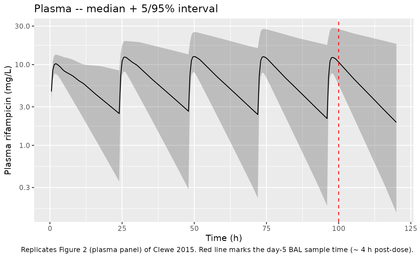
sim_long <- sim |>
  filter(time > 0) |>
  select(id, time, Cc, Celf, Cac) |>
  pivot_longer(c(Cc, Celf, Cac), names_to = "compartment", values_to = "conc") |>
  mutate(compartment = recode(compartment, Cc = "Plasma", Celf = "ELF", Cac = "AC")) |>
  group_by(time, compartment) |>
  summarise(
    Q05 = quantile(conc, 0.05, na.rm = TRUE),
    Q50 = quantile(conc, 0.50, na.rm = TRUE),
    Q95 = quantile(conc, 0.95, na.rm = TRUE),
    .groups = "drop"
  )

ggplot(sim_long, aes(time, Q50, colour = compartment, fill = compartment)) +
  geom_ribbon(aes(ymin = Q05, ymax = Q95), alpha = 0.2, colour = NA) +
  geom_line() +
  geom_vline(xintercept = 100, colour = "grey20", linetype = "dashed") +
  scale_y_log10() +
  labs(x = "Time (h)", y = "Rifampicin concentration (mg/L)",
       title = "Plasma, ELF, and AC -- median + 5/95% interval",
       caption = "Replicates Figure 2 of Clewe 2015. Dashed line at t = 100 h (~ 4 h post the day-5 dose) is the BAL sampling time.")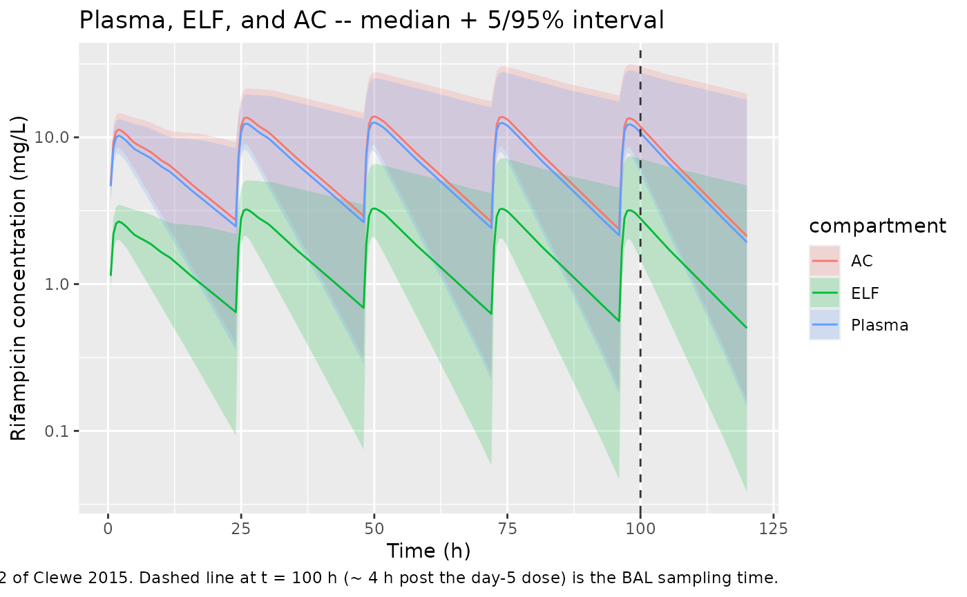
Replicate the published distribution ratios
At pseudo steady-state the model is parameterised to give R_ELF/plasma = 0.26 and R_AC/plasma = 1.1; after dividing by the 20% rifampicin plasma free fraction (fu = 0.20) the unbound ratios are 1.28 and 5.5 (Clewe 2015 Table 1, footnotes b/c). Compute the same ratios from the typical-value simulation at the day-5 BAL time:
mod_typical <- mod |> rxode2::zeroRe()
#> ℹ parameter labels from comments will be replaced by 'label()'
sim_typical <- rxode2::rxSolve(mod_typical, events = events,
                               keep = c("WT", "HT", "FFM", "SEXF"))
#> ℹ omega/sigma items treated as zero: 'etalcl'
#> Warning: multi-subject simulation without without 'omega'

ratios_4h <- sim_typical |>
  filter(time == 100) |>
  summarise(
    R_ELF_plasma         = mean(Celf / Cc),
    R_AC_plasma          = mean(Cac  / Cc),
    R_ELF_unbound_plasma = mean(Celf / Cc) / 0.20,
    R_AC_unbound_plasma  = mean(Cac  / Cc) / 0.20
  )

knitr::kable(
  bind_rows(
    tibble(quantity = "R_ELF/plasma",         published = 0.26, simulated = ratios_4h$R_ELF_plasma),
    tibble(quantity = "R_AC/plasma",          published = 1.10, simulated = ratios_4h$R_AC_plasma),
    tibble(quantity = "R_ELF/unbound-plasma", published = 1.28, simulated = ratios_4h$R_ELF_unbound_plasma),
    tibble(quantity = "R_AC/unbound-plasma",  published = 5.50, simulated = ratios_4h$R_AC_unbound_plasma)
  ),
  digits = 3,
  caption = "Simulated steady-state ELF/plasma and AC/plasma ratios at the day-5 BAL time vs Clewe 2015 Table 1."
)| quantity | published | simulated |
|---|---|---|
| R_ELF/plasma | 0.26 | 0.260 |
| R_AC/plasma | 1.10 | 1.102 |
| R_ELF/unbound-plasma | 1.28 | 1.302 |
| R_AC/unbound-plasma | 5.50 | 5.510 |
PKNCA validation
Use PKNCA to compute Cmax, Tmax, AUC, and half-life for the plasma
compartment over the 24-h interval following the day-5 dose. Because the
cohort received a single regimen (600 mg po qd), the treatment grouping
in the formula is a single regimen label so the PKNCA
result is one summary row per analysis interval (compatible with
multi-regimen extensions in the future).
sim_nca <- sim |>
  as.data.frame() |>
  dplyr::filter(!is.na(Cc), time >= 96, time <= 120) |>
  dplyr::distinct(id, time, .keep_all = TRUE) |>          # multi-output sim has 3 rows per (id,time)
  dplyr::mutate(regimen = "600 mg po qd",
                time = time - 96) |>                       # zero-time at last dose
  dplyr::transmute(id, time, Cc, regimen)

dose_nca <- events |>
  dplyr::filter(evid == 1L, time == 96) |>
  dplyr::distinct(id, time, .keep_all = TRUE) |>
  dplyr::mutate(regimen = "600 mg po qd", time = 0) |>
  dplyr::transmute(id, time, amt, regimen)

conc_obj <- PKNCA::PKNCAconc(sim_nca, Cc ~ time | regimen + id)
dose_obj <- PKNCA::PKNCAdose(dose_nca, amt ~ time | regimen + id)

intervals <- data.frame(
  start       = 0,
  end         = 24,
  cmax        = TRUE,
  tmax        = TRUE,
  auclast     = TRUE,
  half.life   = TRUE
)

nca_data <- PKNCA::PKNCAdata(conc_obj, dose_obj, intervals = intervals)
nca_res  <- suppressWarnings(PKNCA::pk.nca(nca_data))

knitr::kable(
  summary(nca_res),
  caption = "Simulated NCA over the day-5 600 mg po dose interval (regimen-level summary)."
)| start | end | regimen | N | auclast | cmax | tmax | half.life |
|---|---|---|---|---|---|---|---|
| 0 | 24 | 600 mg po qd | 40 | 151 [69.5] | 12.8 [36.3] | 2.00 [1.50, 2.00] | 10.6 [6.58] |
Comparison against published Cmax
Clewe 2015 does not tabulate NCA parameters in the main paper; the underlying Conte 2004 cohort reports a typical 600 mg po qd day-5 plasma Cmax in the 5-10 mg/L range and Tmax 1-4 h. Confirm the simulation Cmax is within this expected range; treat larger discrepancies as a signal to re-check parameter provenance rather than to tune.
Assumptions and deviations
- HIV/AIDS strata not modelled. The original cohort included a 2x2 sex by HIV/AIDS stratification, but Clewe 2015 explicitly chose not to test HIV/AIDS or any other subpopulation indicator as a covariate on the PK (Methods paragraph 1 and Discussion paragraph 5). The model carries no AIDS-related covariate; downstream users who want a stratified analysis should evaluate it on a separate dataset rather than retrofitting the published model.
- Individual demographics are simulated. Clewe 2015 does not reprint the Conte 2004 subject-level WT / HT / SEXF values, so the vignette generates a virtual cohort with the published 50% female sex distribution and plausible adult body-composition ranges (WT ~ N(72, 12) kg, HT ~ N(1.70, 0.09) m). FFM is derived from the simulated WT / HT / SEXF via the Janmahasatian / Anderson-Holford WHSMAX/WHS50 formula reported in Clewe 2015 Eq. 3.
-
kELF and kAC fixed (instantaneous distribution).
The one-BAL-sample-per-subject design did not support estimation of the
distribution rate constants kELF and kAC; both are fixed at 41.58 /h (~
1-minute equilibration half-life, effectively instantaneous at the 4-h
BAL sampling time). For datasets with multiple post-dose BAL samples per
subject, kELF and kAC could be estimated independently and the in-file
fixed()wrapper relaxed. -
No IIV on V/F, MTT, R_ELF/plasma, R_AC/plasma.
Clewe 2015 reports IIV only on CL/F (88.8% CV), with all other PK and
distribution parameters carrying only typical values (Discussion
paragraph 2: “In this analysis example, no IIV was quantified for the
parameters describing the rate or extent of distribution. In order to
allow for IIV to be quantified with good precision, more than one sample
per subject is needed.”). The model file therefore declares
etalclonly. - ELF / AC protein binding assumed negligible. Clewe 2015 Methods paragraph 5 documents this assumption (low protein concentration in ELF observed in paediatric reference studies); the unbound ELF/plasma ratio is derived by dividing R_ELF/plasma by the 20% plasma free fraction without further correction for any ELF/AC protein binding. If a future dataset includes ELF protein quantification, an analogous correction factor could be added.
-
Compartment naming. The ELF and AC effect
compartments are encoded as
effect1andeffect2(canonical numbered-effect-compartment pattern) with observation aliasesCelfandCac; the enzyme-turnover state is encoded asenz_pool(matching the existingSvensson_2016_rifampicinmodel).checkModelConventions()reports a warning forenz_poolbecause it is not a canonical compartment name; the deviation is accepted as the Smythe 2012 / Svensson 2016 / Wilkins 2008 published idiom for rifampicin autoinduction models.