Upadacitinib in ulcerative colitis (Ponce-Bobadilla 2023)
Source:vignettes/articles/PonceBobadilla_2023_upadacitinib.Rmd
PonceBobadilla_2023_upadacitinib.RmdModels and source
Ponce-Bobadilla 2023 re-estimates the cross-population upadacitinib population PK model after adding the ulcerative colitis (UC) phase 2b/3 induction data, then relates the model-estimated steady-state average concentration (Cavg) to efficacy at the end of 8-week induction and of 52-week maintenance with landmark logistic regressions. Following the package’s policy of replicating the authors’ model structure, each fitted model is a separate file and all ten share this vignette.
| Model | Endpoint | Drug term | Source |
|---|---|---|---|
PonceBobadilla_2023_upadacitinib |
plasma concentration | 2-compartment, parallel zero- + first-order absorption | OSM Table 6, OSM Methods |
..._induction_clinrem |
P(clinical remission, Week 8) | log(1 + Cavg) | OSM Table 7 |
..._induction_clinresp |
P(clinical response, Week 8) | log(1 + Cavg) | OSM Table 7 |
..._induction_endoimp |
P(endoscopic improvement, Week 8) | log(1 + Cavg) | OSM Table 7 |
..._induction_endorem |
P(endoscopic remission, Week 8) | log(1 + Cavg) | OSM Table 7 |
..._maintenance_clinrem |
P(clinical remission, Week 52) | log(1 + Cavg) | OSM Table 7 |
..._maintenance_endoimp |
P(endoscopic improvement, Week 52) | log(1 + Cavg) | OSM Table 7 |
..._maintenance_endorem |
P(endoscopic remission, Week 52) | treatment effect | OSM Table 7 |
..._maintenance_hemi |
P(histo-endoscopic mucosal improvement, Week 52) | log(1 + Cavg) | OSM Table 7 |
..._maintenance_sfclinrem |
P(steroid-free clinical remission, Week 52) | log(1 + Cavg) | OSM Table 7 |
- Citation: Ponce-Bobadilla AV, Stodtmann S, Eckert D, Zhou W, Liu W, Mohamed M-EF. Upadacitinib population pharmacokinetics and exposure-response relationships in ulcerative colitis patients. Clin Pharmacokinet. 2023;62(1):101-112. doi:10.1007/s40262-022-01191-6. Parameter values are Supplementary Table 6 of the Online Supplementary Material (OSM); the covariate and residual-error equations are in the OSM Methods.
- Article: https://doi.org/10.1007/s40262-022-01191-6 (open access). Every parameter value is in the Online Supplementary Material (OSM) published with the article.
# readModelDb() returns the model FUNCTION; rxode2::rxode() parses it once.
mod_pk <- rxode2::rxode(readModelDb("PonceBobadilla_2023_upadacitinib"))
#> ℹ parameter labels from comments will be replaced by 'label()'

er_names <- c(
  induction_clinrem = "PonceBobadilla_2023_upadacitinib_induction_clinrem",
  induction_clinresp = "PonceBobadilla_2023_upadacitinib_induction_clinresp",
  induction_endoimp = "PonceBobadilla_2023_upadacitinib_induction_endoimp",
  induction_endorem = "PonceBobadilla_2023_upadacitinib_induction_endorem",
  maintenance_clinrem = "PonceBobadilla_2023_upadacitinib_maintenance_clinrem",
  maintenance_endoimp = "PonceBobadilla_2023_upadacitinib_maintenance_endoimp",
  maintenance_endorem = "PonceBobadilla_2023_upadacitinib_maintenance_endorem",
  maintenance_hemi = "PonceBobadilla_2023_upadacitinib_maintenance_hemi",
  maintenance_sfclinrem = "PonceBobadilla_2023_upadacitinib_maintenance_sfclinrem"
)
mod_er <- lapply(er_names, function(nm) rxode2::rxode(readModelDb(nm)))
Population
The PK analysis pooled 1,927 subjects: phase 1 healthy volunteers, phase 2b patients with rheumatoid arthritis, Crohn’s disease, atopic dermatitis and UC, and the phase 3 UC induction trials. 978 UC patients from induction Studies 1, 2 and 4 contributed to the estimation; 623 patients from maintenance Study 3 were used for a post hoc validation. Among the 978 UC induction patients (OSM Table 3) mean age was 42.9 years, mean body weight 73.1 kg (SD 18.3), 38% were female, 69% White and 26% Asian, 58% were biologic-intolerant or inadequate responders (Bio-IR), mean creatinine clearance was 112 mL/min (SD 32.9) and mean AST 17.9 IU/L. Every UC patient received the extended-release tablet once daily: 7.5, 15, 30 or 45 mg for induction (7.5-30 mg only in the phase 2b Study 1), 15 or 30 mg for maintenance.
The induction exposure-response analysis used 1,234 UC patients (placebo or upadacitinib; Study 1 248, Study 2 472, Study 4 514) and the maintenance analysis 449 patients of Study 3, all of them clinical responders to 45 mg once-daily induction, randomized to placebo, 15 or 30 mg.
str(readModelDb("PonceBobadilla_2023_upadacitinib")()$population, max.level = 1)
#> List of 12
#>  $ species                : chr "human"
#>  $ n_subjects             : int 1927
#>  $ age_range              : chr "Not tabulated for the pooled dataset; ulcerative colitis induction patients mean 42.9 years (SD 14.4; OSM Table 3)."
#>  $ weight_range           : chr "Not tabulated for the pooled dataset; ulcerative colitis induction patients mean 73.1 kg (SD 18.3; OSM Table 3)."
#>  $ sex_female_pct         : num 38
#>  $ race_ethnicity         : chr "Ulcerative colitis induction patients (N = 978): White 69%, Black or African American 3%, Asian 26%, Other/Mult"| __truncated__
#>  $ disease_state          : chr "Pooled healthy volunteers (phase I) and patients with rheumatoid arthritis, Crohn's disease, atopic dermatitis "| __truncated__
#>  $ dose_range             : chr "Ulcerative colitis: 7.5, 15, 30 or 45 mg once daily extended-release tablet for 8-week induction; 15 or 30 mg o"| __truncated__
#>  $ regions                : chr "Multinational; 22% of ulcerative colitis induction patients from the US and 23% from Asian regions (OSM Table 3)."
#>  $ sex_female_pct_note    : chr "38% female among ulcerative colitis induction (N = 978) and maintenance (N = 623) PK patients (OSM Tables 3-4);"| __truncated__
#>  $ crcl_ulcerative_colitis: chr "Mean 112 mL/min (SD 32.9) in induction patients (OSM Table 3); median 109 mL/min (range 42.0-290) in maintenanc"| __truncated__
#>  $ notes                  : chr "NONMEM 7.4.4, FOCE with interaction. All parameters of the Nader 2020 cross-population model were re-estimated "| __truncated__
Source trace
Every ini() value carries an in-file comment naming its
source. They are collected here.
Population pharmacokinetics
(PonceBobadilla_2023_upadacitinib)
| Parameter | Value | Source location |
|---|---|---|
lcl (CL/F) |
37.0 L/h | OSM Table 6 |
lvc (Vc/F) |
169 L | OSM Table 6 |
lq (Q/F) |
3.86 L/h | OSM Table 6 (row label merged with the preceding row) |
lvp (Vp/F) |
61.6 L | OSM Table 6 |
lka_er |
0.114 1/h | OSM Table 6 ‘Extended-Release KA’ |
ltlag_er |
0.159 h | OSM Table 6 ‘Extended-Release Absorption Lag Time’ |
logitffo |
first-order share 27.5% | OSM Table 6 ‘Fraction … Absorbed through Zero-Order Process’ = 72.5% |
ld2 |
3.39 h | OSM Table 6 ‘Zero-Order Absorption Duration’ |
lfrel_er |
79.8% | OSM Table 6 ‘Bioavailability of the Extended-Release …’ |
lka_ir |
1.85 1/h | OSM Table 6 ‘Immediate-Release KA’ |
ltlag_ir |
0.237 h | OSM Table 6 ‘Immediate-Release Absorption Lag Time’ |
e_crcl_cl |
0.213 | OSM Table 6 |
e_ast_cl |
-0.0810 | OSM Table 6 |
e_sexf_cl |
log(0.874) | OSM Table 6 ‘CL/F Ratio of Females Compared to Males’ |
e_dis_healthy_cl |
log(1.22) | OSM Table 6 ‘CL/F Ratio of Healthy Patients …’ |
e_dis_ra_cl |
log(0.929) | OSM Table 6 ‘CL/F Ratio of RA Patients …’ |
e_wt_vc |
0.493 | OSM Table 6 |
e_sexf_vc |
log(0.811) | OSM Table 6 ‘Vc/F Ratio of Females Compared to Males’ |
etalcl, etalvc
|
34.5%, 27.0% | OSM Table 6 ISV, as 100 * sqrt(omega^2) |
etalka_er, etalka_ir
|
94.3%, 71.4% | OSM Table 6 ISV |
propSdPhase1, propSdPhase23
|
0.261, 0.456 | OSM Table 6 |
addSdBase |
0.115 ng/mL | OSM Table 6 |
ruv_early |
1.68 | OSM Table 6 ‘Scaling Factor on Residual Error’; OSM Supplementary Results (first 2 h after dosing) |
| Covariate equation | power / exp(cov * theta) | OSM Methods ‘Population pharmacokinetic modeling’ |
| Residual-error form | C = Chat (1 + eps_Phase) + eps_ADD | OSM Methods |
| Absorption structure, lag on first-order arm | n/a | main text Section 2.3 |
| Reference WT / CrCL / AST | 70 kg / 109 mL/min / 18 IU/L | not printed; see Assumptions and deviations |
Exposure-response (..._induction_*,
..._maintenance_*)
All coefficients are OSM Table 7; the model form is the OSM Methods equation logit P = alpha + f(Cavg) + sum(betaj xj), with f(C) = beta log(1 + C) for the logarithmic models and betatrt for the treatment-effect model.
| Model | Intercept | log(1 + Cavg) or treatment | Bio-IR | Steroid | Adapted Mayo > 7 / Remission at Wk 0 | Study 2 | Study 4 |
|---|---|---|---|---|---|---|---|
| induction clinrem | -3.07 | 0.636 | -0.776 | -0.0375 | -0.363 | 0.154 | 0.481 |
| induction clinresp | -1.41 | 0.598 | -1.04 | 0.176 | 0.387 | 0.539 | 0.581 |
| induction endoimp | -2.17 | 0.593 | -0.922 (see Errata) | 0.201 | -0.241 | -0.188 | 0.152 |
| induction endorem | -3.69 | 0.658 | -1.07 | 0.321 | -0.133 | -0.276 | 0.0624 |
| maintenance clinrem | -2.22 | 0.57 | -0.156 | -0.121 | 1.02 | – | – |
| maintenance endoimp | -1.95 | 0.632 | -0.41 | -0.0944 | 0.913 | – | – |
| maintenance endorem | -3.1 | 1.75 (treatment) | -0.277 | -0.444 | 1.04 | – | – |
| maintenance hemi | -2.4 | 0.526 | -0.0883 | -0.138 | 1.01 | – | – |
| maintenance sfclinrem | -2.24 | 0.561 | -0.0667 | -0.367 | 1.04 | – | – |
Virtual cohort
Observed data are not public. The PK cohort approximates the UC induction PK population of OSM Table 3, with 200 subjects in each of the four dose groups.
# set.seed() fixes the covariate draws; rxode2's own between-subject draws
# depend on the solver thread layout, so every assertion below is on medians,
# means or structural identities, never on the extremes of the cohort.
set.seed(20221226)
rxode2::rxSetSeed(20221226)

N_ARM <- 200L
DOSES <- c(7.5, 15, 30, 45)

pk_subjects <- tibble(
  id = seq_len(N_ARM * length(DOSES)),
  dose = rep(DOSES, each = N_ARM),
  # OSM Table 3, all UC induction patients: weight mean 73.1 (SD 18.3) kg,
  # 38% female, CrCL mean 112 (SD 32.9) mL/min, AST mean 17.9 IU/L.
  WT = pmin(pmax(rnorm(N_ARM * length(DOSES), 73.1, 18.3), 40), 160),
  SEXF = rbinom(N_ARM * length(DOSES), 1L, 0.38),
  CRCL = pmin(pmax(rnorm(N_ARM * length(DOSES), 112, 32.9), 42), 290),
  AST = pmin(pmax(exp(rnorm(N_ARM * length(DOSES), log(16), 0.3)), 5), 150),
  DIS_HEALTHY = 0, DIS_RA = 0, FORM_UPA_ER = 1, STUDY_UPA_PHASE1 = 0
) |>
  mutate(arm = factor(paste(dose, "mg QD"), levels = paste(DOSES, "mg QD")))

summary(pk_subjects[, c("WT", "CRCL", "AST")])
#>        WT              CRCL             AST
#>  Min.   : 40.00   Min.   : 42.00   Min.   : 5.00
#>  1st Qu.: 60.66   1st Qu.: 89.31   1st Qu.:12.91
#>  Median : 74.58   Median :112.25   Median :15.68
#>  Mean   : 74.43   Mean   :112.25   Mean   :16.59
#>  3rd Qu.: 87.11   3rd Qu.:135.84   3rd Qu.:19.31
#>  Max.   :125.58   Max.   :208.94   Max.   :38.44
Event table
The extended-release absorption is a parallel
process, so each administration is two dose records at the same time:
one into depot (the first-order arm, scaled by
f(depot)) and one into central with
rate = -2 (the zero-order arm over the modelled
dur(central)). Observations point at the ODE state
central; Cc is returned alongside.
DOSE_TIMES <- seq(0, 144, by = 24) # seven once-daily doses
OBS_TIMES <- seq(144, 168, by = 0.25) # the seventh dosing interval

expand_rows <- function(df, times) df[rep(seq_len(nrow(df)), each = length(times)), ]

depot_doses <- expand_rows(pk_subjects, DOSE_TIMES) |>
  mutate(time = rep(DOSE_TIMES, nrow(pk_subjects)), amt = dose, evid = 1L,
         cmt = "depot", rate = 0)
central_doses <- depot_doses |> mutate(cmt = "central", rate = -2)
observations <- expand_rows(pk_subjects, OBS_TIMES) |>
  mutate(time = rep(OBS_TIMES, nrow(pk_subjects)), amt = NA_real_, evid = 0L,
         cmt = "central", rate = 0)

events <- bind_rows(depot_doses, central_doses, observations) |>
  select(id, time, amt, evid, cmt, rate, everything()) |>
  arrange(id, time, desc(evid))

stopifnot(length(unique(events$id)) == N_ARM * length(DOSES))Replicate published figures
# Shape of Figure 2 of Ponce-Bobadilla 2023 (visual predictive check by
# induction dose group, versus time after the last dose).
sim |>
  mutate(tad = time - max(DOSE_TIMES)) |>
  group_by(arm, tad) |>
  summarise(Q05 = quantile(Cc, 0.05), Q50 = median(Cc), Q95 = quantile(Cc, 0.95),
            .groups = "drop") |>
  ggplot(aes(tad, Q50)) +
  geom_ribbon(aes(ymin = Q05, ymax = Q95), alpha = 0.2, fill = "steelblue") +
  geom_line(colour = "purple4", linewidth = 0.8) +
  facet_wrap(~arm, scales = "free_y") +
  scale_x_continuous(breaks = seq(0, 24, by = 4)) +
  labs(x = "Time after last dose (h)", y = "Upadacitinib concentration (ng/mL)",
       caption = paste("Simulated median and 90% prediction interval at steady state.",
                       "Compare with Figure 2 of Ponce-Bobadilla 2023."))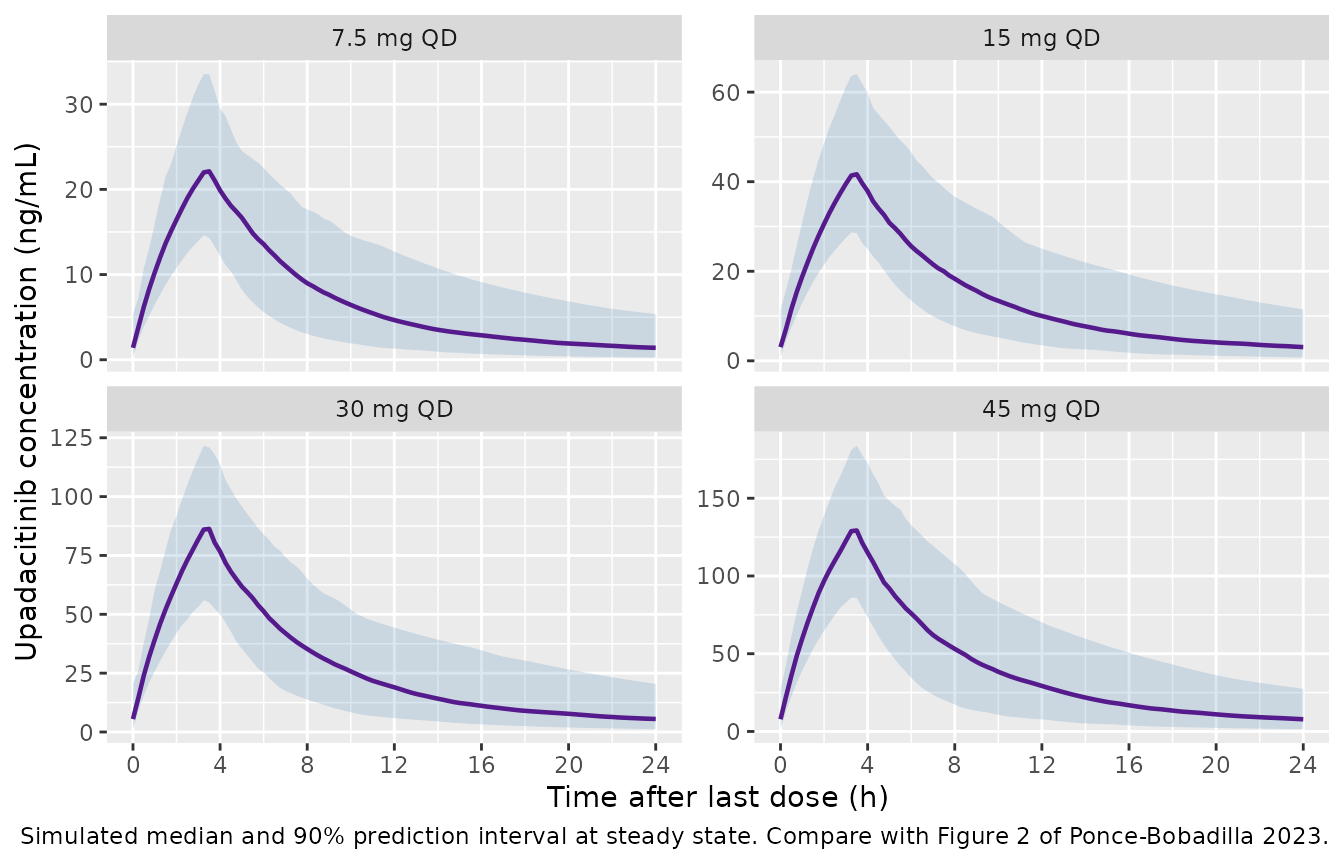
PKNCA validation
Steady-state NCA over the seventh dosing interval. The half-life is not requested: the extended-release first-order arm absorbs with a 6 h half-life and 94% IIV, so a 24 h window cannot separate absorption from elimination.
sim_nca <- sim |>
  dplyr::filter(!is.na(Cc)) |>
  dplyr::select(id, time, Cc, arm)

conc_obj <- PKNCA::PKNCAconc(sim_nca, Cc ~ time | arm + id)
dose_df <- events |>
  dplyr::filter(evid == 1, cmt == "depot") |>
  dplyr::select(id, time, amt, arm)
dose_obj <- PKNCA::PKNCAdose(dose_df, amt ~ time | arm + id)

intervals <- data.frame(start = 144, end = 168, cmax = TRUE, tmax = TRUE,
                        auclast = TRUE, cav = TRUE)
nca_res <- PKNCA::pk.nca(PKNCA::PKNCAdata(conc_obj, dose_obj, intervals = intervals))Ctrough in OSM Table 5 is the pre-dose concentration at
steady state, so it is read directly off the profile at the end of the
interval rather than taken from cmin; the 0.159 h lag puts
the interval minimum just after the dose.
ctrough_df <- sim |>
  dplyr::filter(time == max(OBS_TIMES)) |>
  dplyr::transmute(arm, id, PPTESTCD = "ctrough", PPORRES = Cc)

nca_long <- dplyr::bind_rows(
  as.data.frame(nca_res)[, c("arm", "id", "PPTESTCD", "PPORRES")],
  ctrough_df
)
stopifnot(!anyNA(nca_long$PPORRES))
Comparison against OSM Table 5
OSM Table 5 gives model-estimated steady-state exposures in UC patients by dose group, as median (5th, 95th percentile) of the post hoc estimates.
published <- tibble::tribble(
  ~arm,       ~cav,  ~cmax, ~ctrough,
  "7.5 mg QD", 6.69, 20.2,  1.06,
  "15 mg QD",  14.3, 41.3,  2.63,
  "30 mg QD",  27.2, 78.5,  4.94,
  "45 mg QD",  41.4, 121,   7.08
) |>
  mutate(arm = factor(arm, levels = levels(pk_subjects$arm)))

cmp <- nlmixr2lib::ncaComparisonTable(
  simulated = nca_long |> dplyr::filter(PPTESTCD %in% c("cav", "cmax", "ctrough")),
  reference = published,
  by = "arm",
  units = c(cav = "ng/mL", cmax = "ng/mL", ctrough = "ng/mL"),
  tolerance_pct = 20
)
knitr::kable(cmp, caption = "Simulated vs. OSM Table 5 (medians). * differs by >20%.")| NCA parameter | arm | Reference | Simulated | % diff |
|---|---|---|---|---|
| Cmax (ng/mL) | 7.5 mg QD | 20.2 | 22.2 | +10.0% |
| Cmax (ng/mL) | 15 mg QD | 41.3 | 41.7 | +0.9% |
| Cmax (ng/mL) | 30 mg QD | 78.5 | 86.9 | +10.7% |
| Cmax (ng/mL) | 45 mg QD | 121 | 130 | +7.1% |
| Cavg (ng/mL) | 7.5 mg QD | 6.69 | 7.26 | +8.5% |
| Cavg (ng/mL) | 15 mg QD | 14.3 | 14.2 | -0.8% |
| Cavg (ng/mL) | 30 mg QD | 27.2 | 27.9 | +2.5% |
| Cavg (ng/mL) | 45 mg QD | 41.4 | 41.4 | -0.1% |
| Ctrough (ng/mL) | 7.5 mg QD | 1.06 | 1.4 | +32.3%* |
| Ctrough (ng/mL) | 15 mg QD | 2.63 | 3.06 | +16.4% |
| Ctrough (ng/mL) | 30 mg QD | 4.94 | 5.53 | +11.9% |
| Ctrough (ng/mL) | 45 mg QD | 7.08 | 7.85 | +10.9% |
gate <- nca_long |>
  group_by(arm, PPTESTCD) |>
  summarise(median = median(PPORRES), .groups = "drop") |>
  tidyr::pivot_wider(names_from = PPTESTCD, values_from = median) |>
  dplyr::left_join(published, by = "arm", suffix = c("_sim", "_pub")) |>
  mutate(pct_cav = 100 * (cav_sim / cav_pub - 1),
         pct_cmax = 100 * (cmax_sim / cmax_pub - 1),
         pct_ctrough = 100 * (ctrough_sim / ctrough_pub - 1))

# The PK is linear, so the four arms differ only by dose and by which 200
# subjects were drawn; a per-arm median of C_trough (5th-95th percentile spans
# a factor of ten) moves by 10-20% between draws. The gate therefore pools the
# dose-normalized exposures of all 800 subjects and compares the median with
# the 45 mg arm of OSM Table 5 (n = 771, the most precise row). A
# mis-transcribed clearance, bioavailability, dose or unit moves these by tens
# of percent. Observed when written: C_avg +2%, C_max +6%, C_trough +20%
# (forward-simulated troughs sit above the shrunken post hoc ones; the
# typical-value trough alone is +7%).
pooled <- nca_long |>
  dplyr::filter(PPTESTCD %in% c("cav", "cmax", "ctrough")) |>
  mutate(id = as.integer(as.character(id))) |>
  dplyr::left_join(dplyr::distinct(sim, id, dose), by = "id") |>
  group_by(PPTESTCD) |>
  summarise(per_mg = median(PPORRES / dose), .groups = "drop")
pub_per_mg <- c(cav = 41.4, cmax = 121, ctrough = 7.08) / 45
pooled$pct <- 100 * (pooled$per_mg / pub_per_mg[pooled$PPTESTCD] - 1)
pooled
#> # A tibble: 3 × 3
#>   PPTESTCD per_mg   pct
#>   <chr>     <dbl> <dbl>
#> 1 cav       0.939  2.02
#> 2 cmax      2.86   6.25
#> 3 ctrough   0.188 19.8
stopifnot(
  abs(pooled$pct[pooled$PPTESTCD == "cav"]) < 10,
  abs(pooled$pct[pooled$PPTESTCD == "cmax"]) < 20,
  abs(pooled$pct[pooled$PPTESTCD == "ctrough"]) < 30
)
# Dose proportionality (main text Section 3.1): C_avg per mg is flat across arms.
cav_per_mg <- gate$cav_sim / DOSES
stopifnot(max(cav_per_mg) / min(cav_per_mg) < 1.1)

gate |>
  dplyr::select(arm, pct_cav, pct_cmax, pct_ctrough) |>
  mutate(across(where(is.numeric), ~ round(., 1))) |>
  dplyr::rename("Dose group" = arm, "C_avg (%)" = pct_cav, "C_max (%)" = pct_cmax,
                "C_trough (%)" = pct_ctrough) |>
knitr::kable(caption = "Percent difference of the simulated median from OSM Table 5.")| Dose group | C_avg (%) | C_max (%) | C_trough (%) |
|---|---|---|---|
| 7.5 mg QD | 8.5 | 10.0 | 32.3 |
| 15 mg QD | -0.8 | 0.9 | 16.4 |
| 30 mg QD | 2.5 | 10.7 | 11.9 |
| 45 mg QD | -0.1 | 7.1 | 10.9 |
tmax_med <- nca_long |>
  dplyr::filter(PPTESTCD == "tmax") |>
  group_by(arm) |>
  summarise(tmax = median(PPORRES), .groups = "drop")
tmax_med
#> # A tibble: 4 × 2
#>   arm        tmax
#>   <fct>     <dbl>
#> 1 7.5 mg QD   3.5
#> 2 15 mg QD    3.5
#> 3 30 mg QD    3.5
#> 4 45 mg QD    3.5
The published percentiles come from post hoc empirical Bayes estimates under sparse sampling (three or four samples per patient), so they are compressed relative to a forward simulation for the absorption parameters with large IIV; only the medians are gated.
Internal structural identities
At steady state C_avg = F_rel x Dose / (CL/F x tau),
which is exactly how the OSM computes the exposure metric for the
exposure-response models. The typical-value check has no random draw, so
its bound is tight.
typical <- tibble(id = 1:6, WT = c(50, 70, 110, 70, 70, 70),
                  CRCL = c(109, 109, 109, 60, 180, 109),
                  AST = c(18, 18, 18, 18, 18, 40), SEXF = c(0, 0, 0, 1, 0, 0),
                  DIS_HEALTHY = 0, DIS_RA = 0, FORM_UPA_ER = 1, STUDY_UPA_PHASE1 = 0)
typ_events <- bind_rows(
  expand_rows(typical, DOSE_TIMES) |>
    mutate(time = rep(DOSE_TIMES, nrow(typical)), amt = 45, evid = 1L, cmt = "depot", rate = 0),
  expand_rows(typical, DOSE_TIMES) |>
    mutate(time = rep(DOSE_TIMES, nrow(typical)), amt = 45, evid = 1L, cmt = "central", rate = -2),
  expand_rows(typical, OBS_TIMES) |>
    mutate(time = rep(OBS_TIMES, nrow(typical)), amt = NA_real_, evid = 0L, cmt = "central", rate = 0)
) |>
  select(id, time, amt, evid, cmt, rate, everything()) |>
  arrange(id, time, desc(evid))

# zeroRe() removes the random effects on purpose; rxode2 notes it.
typ_chk <- suppressWarnings(as.data.frame(rxode2::rxSolve(rxode2::zeroRe(mod_pk), typ_events))) |>
  group_by(id) |>
  summarise(cav = sum(diff(time) * (head(Cc, -1) + tail(Cc, -1)) / 2) / 24,
            cl = first(cl), .groups = "drop") |>
  mutate(pct = 100 * (cav / (0.798 * 45 * 1000 / (cl * 24)) - 1))
#> ℹ omega/sigma items treated as zero: 'etalcl', 'etalvc', 'etalka_er', 'etalka_ir'
stopifnot(max(abs(typ_chk$pct)) < 0.5)
signif(typ_chk$pct, 3)
#> [1] -0.0426 -0.0366 -0.0302 -0.0363 -0.0400 -0.0348

# The reference subject (row 2) has CL/F = 37.0 L/h exactly.
stopifnot(abs(typ_chk$cl[2] - 37.0) < 1e-6)
Across the full cohort the same identity holds on the centre of the distribution; subjects drawing a very slow extended-release Ka are still approaching steady state at day 7, which puts a tail on the deviation.
cl_per_id <- sim |> group_by(id) |> summarise(cl = first(cl), dose = first(dose), .groups = "drop")
cav_chk <- nca_long |>
  dplyr::filter(PPTESTCD == "cav") |>
  mutate(id = as.integer(as.character(id))) |>
  dplyr::left_join(cl_per_id, by = "id") |>
  mutate(pct = 100 * (PPORRES / (0.798 * dose * 1000 / (cl * 24)) - 1))
# Observed when written: median 0.06%, 90th percentile 0.23%.
stopifnot(abs(median(cav_chk$pct)) < 1, quantile(abs(cav_chk$pct), 0.9) < 5)
signif(quantile(abs(cav_chk$pct), c(0.5, 0.9)), 3)
#>    50%    90%
#> 0.0573 0.2300
# FORM_UPA_ER changes only absorption, so AUC(ER) / AUC(IR) after the same
# single dose equals the relative bioavailability 0.798.
single_dose <- function(form, id_offset) {
  s <- tibble(id = id_offset + 1:2, WT = c(60, 90), CRCL = c(90, 130), AST = c(15, 25),
              SEXF = c(1, 0), DIS_HEALTHY = 0, DIS_RA = 0, FORM_UPA_ER = form,
              STUDY_UPA_PHASE1 = 0)
  ot <- seq(0, 240, by = 0.05)
  dep <- s |> mutate(time = 0, amt = 30, evid = 1L, cmt = "depot", rate = 0)
  obs <- s[rep(1:2, each = length(ot)), ] |>
    mutate(time = rep(ot, 2), amt = NA_real_, evid = 0L, cmt = "central", rate = 0)
  ev <- if (form == 1) bind_rows(dep, dep |> mutate(cmt = "central", rate = -2), obs) else bind_rows(dep, obs)
  ev |> select(id, time, amt, evid, cmt, rate, everything()) |> arrange(id, time, desc(evid))
}
trapz_auc <- function(d) {
  d |> group_by(id) |>
    summarise(auc = sum(diff(time) * (head(Cc, -1) + tail(Cc, -1)) / 2), .groups = "drop")
}
mod_typ <- rxode2::zeroRe(mod_pk)
#> Warning: No sigma parameters in the model
auc_er <- suppressWarnings(as.data.frame(rxode2::rxSolve(mod_typ, single_dose(1, 0L)))) |> trapz_auc()
#> ℹ omega/sigma items treated as zero: 'etalcl', 'etalvc', 'etalka_er', 'etalka_ir'
auc_ir <- suppressWarnings(as.data.frame(rxode2::rxSolve(mod_typ, single_dose(0, 10L)))) |> trapz_auc()
#> ℹ omega/sigma items treated as zero: 'etalcl', 'etalvc', 'etalka_er', 'etalka_ir'
frel <- auc_er$auc / auc_ir$auc
stopifnot(max(abs(frel - 0.798)) < 0.005)
round(frel, 4)
#> [1] 0.798 0.798
# The residual error is inflated by 1.68 in the first 2 h after each dose.
# ruv_scale is an algebraic model variable, so it is returned by rxSolve.
ruv <- suppressWarnings(as.data.frame(rxode2::rxSolve(mod_typ, typ_events |> dplyr::filter(id == 2)))) |>
  mutate(tad = time - max(DOSE_TIMES))
#> ℹ omega/sigma items treated as zero: 'etalcl', 'etalvc', 'etalka_er', 'etalka_ir'
stopifnot(all(abs(ruv$ruv_scale[ruv$tad > 0 & ruv$tad < 2] - 1.68) < 1e-12),
          all(abs(ruv$ruv_scale[ruv$tad > 2] - 1) < 1e-12))
Exposure-response
The exposure-response models take Cavg as an input column,
CAV, in ng/mL (0 for placebo). Here each simulated
subject’s PKNCA cav from the cohort above is fed into the
logistic models, with the pre-specified stratification covariates drawn
as described under Assumptions and
deviations, and the predicted probability is averaged by arm – the
same construction as the paper’s Figures 5 and 6, which resampled
patients’ exposures and covariates by treatment group.
cav_subject <- nca_long |>
  dplyr::filter(PPTESTCD == "cav") |>
  transmute(id = as.integer(as.character(id)), CAV = PPORRES) |>
  dplyr::left_join(cl_per_id |> dplyr::select(id, dose), by = "id")

placebo <- tibble(id = 10000L + seq_len(N_ARM), CAV = 0, dose = 0)
er_base <- bind_rows(placebo, cav_subject) |>
  mutate(arm = factor(ifelse(dose == 0, "Placebo", paste(dose, "mg")),
                      levels = c("Placebo", paste(DOSES, "mg"))),
         time = 0)

n_er <- nrow(er_base)
study <- sample(1:3, n_er, replace = TRUE, prob = c(248, 472, 514))
induction_cov <- er_base |>
  mutate(BIOLOGIC_IR = rbinom(n_er, 1L, 0.58),
         CONMED_STEROID = rbinom(n_er, 1L, 0.406),
         SCORE_AMAYO = sample(5:9, n_er, replace = TRUE, prob = c(0.10, 0.20, 0.30, 0.25, 0.15)),
         STUDY_UPA_UC_S2 = as.integer(study == 2),
         STUDY_UPA_UC_S4 = as.integer(study == 3))

maintenance_cov <- er_base |>
  dplyr::filter(arm %in% c("Placebo", "15 mg", "30 mg")) |>
  mutate(arm = droplevels(arm),
         BIOLOGIC_IR = rbinom(n(), 1L, 0.53),
         CONMED_STEROID = rbinom(n(), 1L, 0.40),
         CLINICAL_REMISSION_BL = rbinom(n(), 1L, 0.35),
         ON_TREATMENT = as.integer(arm != "Placebo"))

# rxSolve() reads a column named `dose` as a dose amount, which would turn
# every active-arm row into a dosing record, so the arm bookkeeping columns are
# dropped before the solve and joined back by id.
predict_arm <- function(model, data) {
  data <- data |> mutate(id = seq_len(n()))
  out <- suppressWarnings(as.data.frame(rxode2::rxSolve(rxode2::zeroRe(model),
                                                        dplyr::select(data, -arm, -dose))))
  prob_col <- grep("^prob_", names(out), value = TRUE)
  stopifnot(nrow(out) == nrow(data))
  tibble(id = as.integer(as.character(out$id)), prob = out[[prob_col]]) |>
    dplyr::left_join(dplyr::select(data, id, arm), by = "id") |>
    group_by(arm) |>
    summarise(pct = 100 * mean(prob), .groups = "drop")
}

er_pred <- bind_rows(lapply(names(mod_er), function(nm) {
  dat <- if (startsWith(nm, "induction")) induction_cov else maintenance_cov
  predict_arm(mod_er[[nm]], dat) |> mutate(model = nm)
}))
Comparison against Figures 5 and 6
Figures 5 and 6 of the paper print the model-predicted percentage of patients achieving each endpoint by treatment group (Figure 6 omits maintenance endoscopic remission, the treatment-effect model).
fig <- tibble::tribble(
  ~model,                  ~arm,      ~fig_pct,
  "induction_clinrem",     "Placebo", 4,  "induction_clinrem",  "7.5 mg", 12,
  "induction_clinrem",     "15 mg",   17, "induction_clinrem",  "30 mg",  24,
  "induction_clinrem",     "45 mg",   28,
  "induction_clinresp",    "Placebo", 23, "induction_clinresp", "7.5 mg", 48,
  "induction_clinresp",    "15 mg",   57, "induction_clinresp", "30 mg",  65,
  "induction_clinresp",    "45 mg",   70,
  "induction_endoimp",     "Placebo", 7,  "induction_endoimp",  "7.5 mg", 20,
  "induction_endoimp",     "15 mg",   26, "induction_endoimp",  "30 mg",  34,
  "induction_endoimp",     "45 mg",   39,
  "induction_endorem",     "Placebo", 2,  "induction_endorem",  "7.5 mg", 6,
  "induction_endorem",     "15 mg",   9,  "induction_endorem",  "30 mg",  13,
  "induction_endorem",     "45 mg",   16,
  "maintenance_clinrem",   "Placebo", 13, "maintenance_clinrem",   "15 mg", 40,
  "maintenance_clinrem",   "30 mg",   48,
  "maintenance_endoimp",   "Placebo", 15, "maintenance_endoimp",   "15 mg", 46,
  "maintenance_endoimp",   "30 mg",   56,
  "maintenance_hemi",      "Placebo", 12, "maintenance_hemi",      "15 mg", 34,
  "maintenance_hemi",      "30 mg",   42,
  "maintenance_sfclinrem", "Placebo", 13, "maintenance_sfclinrem", "15 mg", 39,
  "maintenance_sfclinrem", "30 mg",   47
)

er_cmp <- er_pred |>
  mutate(arm = as.character(arm)) |>
  dplyr::left_join(fig, by = c("model", "arm")) |>
  mutate(diff = pct - fig_pct)

er_cmp |>
  mutate(pct = round(pct, 1), diff = round(diff, 1)) |>
  dplyr::select(model, arm, pct, fig_pct, diff) |>
  dplyr::rename("Model" = model, "Arm" = arm, "Simulated (%)" = pct,
                "Figure 5/6 (%)" = fig_pct, "Difference (pp)" = diff) |>
knitr::kable(caption = "Arm-mean predicted response vs the paper's Figures 5 and 6.")| Model | Arm | Simulated (%) | Figure 5/6 (%) | Difference (pp) |
|---|---|---|---|---|
| induction_clinrem | Placebo | 3.5 | 4 | -0.5 |
| induction_clinrem | 7.5 mg | 12.3 | 12 | 0.3 |
| induction_clinrem | 15 mg | 17.2 | 17 | 0.2 |
| induction_clinrem | 30 mg | 22.6 | 24 | -1.4 |
| induction_clinrem | 45 mg | 26.6 | 28 | -1.4 |
| induction_clinresp | Placebo | 22.4 | 23 | -0.6 |
| induction_clinresp | 7.5 mg | 50.0 | 48 | 2.0 |
| induction_clinresp | 15 mg | 58.1 | 57 | 1.1 |
| induction_clinresp | 30 mg | 64.1 | 65 | -0.9 |
| induction_clinresp | 45 mg | 69.6 | 70 | -0.4 |
| induction_endoimp | Placebo | 6.9 | 7 | -0.1 |
| induction_endoimp | 7.5 mg | 20.3 | 20 | 0.3 |
| induction_endoimp | 15 mg | 26.7 | 26 | 0.7 |
| induction_endoimp | 30 mg | 33.2 | 34 | -0.8 |
| induction_endoimp | 45 mg | 36.8 | 39 | -2.2 |
| induction_endorem | Placebo | 1.6 | 2 | -0.4 |
| induction_endorem | 7.5 mg | 6.1 | 6 | 0.1 |
| induction_endorem | 15 mg | 8.9 | 9 | -0.1 |
| induction_endorem | 30 mg | 12.1 | 13 | -0.9 |
| induction_endorem | 45 mg | 14.3 | 16 | -1.7 |
| maintenance_clinrem | Placebo | 12.4 | 13 | -0.6 |
| maintenance_clinrem | 15 mg | 39.7 | 40 | -0.3 |
| maintenance_clinrem | 30 mg | 48.2 | 48 | 0.2 |
| maintenance_endoimp | Placebo | 13.4 | 15 | -1.6 |
| maintenance_endoimp | 15 mg | 46.2 | 46 | 0.2 |
| maintenance_endoimp | 30 mg | 56.1 | 56 | 0.1 |
| maintenance_endorem | Placebo | 4.8 | NA | NA |
| maintenance_endorem | 15 mg | 22.6 | NA | NA |
| maintenance_endorem | 30 mg | 22.7 | NA | NA |
| maintenance_hemi | Placebo | 10.9 | 12 | -1.1 |
| maintenance_hemi | 15 mg | 33.7 | 34 | -0.3 |
| maintenance_hemi | 30 mg | 41.1 | 42 | -0.9 |
| maintenance_sfclinrem | Placebo | 11.8 | 13 | -1.2 |
| maintenance_sfclinrem | 15 mg | 37.9 | 39 | -1.1 |
| maintenance_sfclinrem | 30 mg | 45.8 | 47 | -1.2 |
chk <- er_cmp |> dplyr::filter(!is.na(fig_pct))
# Each simulated value is a mean over 200 subjects, so it is a centre
# statistic; the residual gap reflects the assumed covariate mix.
# Observed when written: median |difference| 0.6, maximum 2.2 points.
stopifnot(
  nrow(chk) == 32,
  median(abs(chk$diff)) < 3,
  all(abs(chk$diff) < 7)
)
# Main-text claims: 45 mg is 3-5 points above 30 mg at induction Week 8, and
# 30 mg is 8-10 points above 15 mg for the four maintenance endpoints of Fig 6.
gain <- er_pred |>
  dplyr::filter(arm %in% c("15 mg", "30 mg", "45 mg")) |>
  tidyr::pivot_wider(names_from = arm, values_from = pct)
ind_gain <- with(dplyr::filter(gain, startsWith(model, "induction")), `45 mg` - `30 mg`)
mai_gain <- with(dplyr::filter(gain, model %in% fig$model, startsWith(model, "maintenance")), `30 mg` - `15 mg`)
# Observed when written: induction 2.2-5.5, maintenance 7.4-9.8 points.
stopifnot(all(ind_gain > 1 & ind_gain < 7), all(mai_gain > 5 & mai_gain < 13))
round(c(ind_gain, mai_gain), 1)
#> [1] 4.1 5.5 3.6 2.2 8.5 9.8 7.4 8.0
# Maintenance endoscopic remission is a treatment-effect model: 15 and 30 mg
# predict the same rate, and the odds ratio is exp(1.75) exactly.
endorem <- er_pred |> dplyr::filter(model == "maintenance_endorem")
endorem
#> # A tibble: 3 × 3
#>   arm       pct model
#>   <fct>   <dbl> <chr>
#> 1 Placebo  4.79 maintenance_endorem
#> 2 15 mg   22.6  maintenance_endorem
#> 3 30 mg   22.7  maintenance_endorem
stopifnot(abs(endorem$pct[endorem$arm == "15 mg"] - endorem$pct[endorem$arm == "30 mg"]) < 3)

ref <- data.frame(id = 1:2, time = 0, BIOLOGIC_IR = 0, CONMED_STEROID = 0,
                  CLINICAL_REMISSION_BL = 0, ON_TREATMENT = c(0, 1))
p <- suppressWarnings(as.data.frame(rxode2::rxSolve(rxode2::zeroRe(mod_er$maintenance_endorem), ref)))$prob_endorem
stopifnot(abs(log(p[2] / (1 - p[2])) - log(p[1] / (1 - p[1])) - 1.75) < 1e-8)
# Shape of Figures 3 and 4: probability against C_avg for a reference patient
# (non-Bio-IR, no corticosteroids, Adapted Mayo <= 7, Study 1 at induction;
# not in remission at maintenance Week 0).
grid <- tibble(id = 1:61, time = 0, CAV = seq(0, 60, by = 1), BIOLOGIC_IR = 0,
               CONMED_STEROID = 0, SCORE_AMAYO = 6, STUDY_UPA_UC_S2 = 0,
               STUDY_UPA_UC_S4 = 0, CLINICAL_REMISSION_BL = 0)
curves <- bind_rows(lapply(setdiff(names(mod_er), "maintenance_endorem"), function(nm) {
  out <- suppressWarnings(as.data.frame(rxode2::rxSolve(rxode2::zeroRe(mod_er[[nm]]), grid)))
  tibble(model = nm, CAV = grid$CAV, prob = out[[grep("^prob_", names(out), value = TRUE)]])
}))
ggplot(curves, aes(CAV, 100 * prob, colour = model)) +
  geom_line(linewidth = 0.8) +
  labs(x = "Upadacitinib C_avg (ng/mL)", y = "Predicted responders (%)", colour = NULL,
       caption = "Reference patient. Compare with Figures 3 and 4 of Ponce-Bobadilla 2023.") +
  theme(legend.position = "bottom") +
  guides(colour = guide_legend(ncol = 2))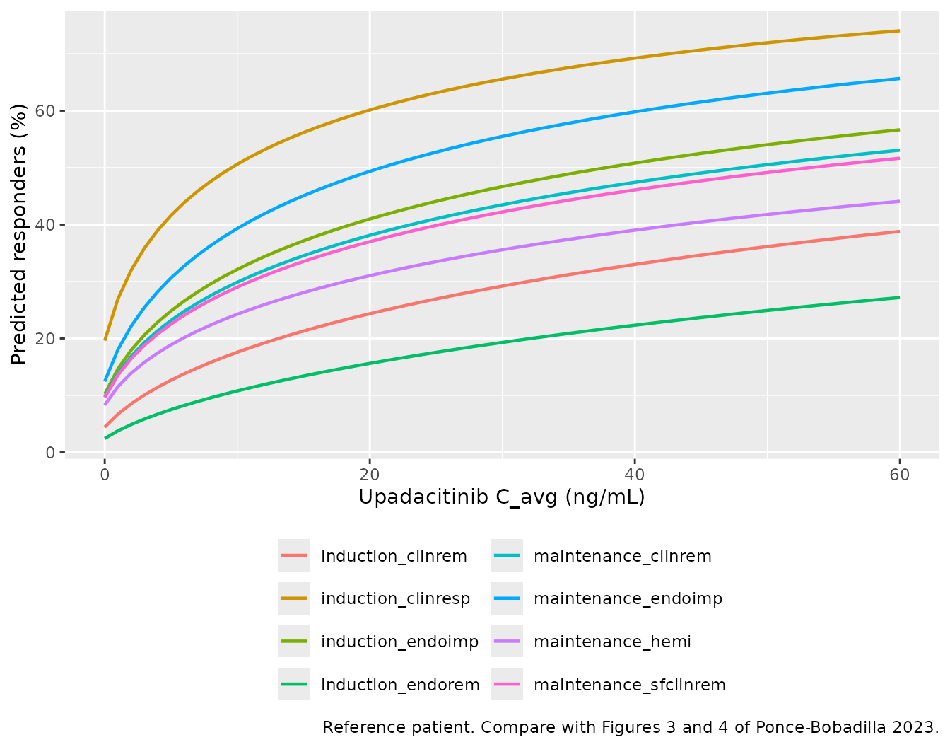
Assumptions and deviations
- Covariate reference values. The OSM Methods normalize continuous PK covariates to “the median of the population”, but the medians of the pooled 1,927-subject dataset are not printed. The model uses values the paper does print: 70 kg (the 70.35 kg median body weight of the UC exposure-response population, OSM Table 8), 109 mL/min (median creatinine clearance of the maintenance PK population, OSM Table 4; the 108.70 mL/min centering of the predecessor Klunder 2019 model agrees) and 18 IU/L (rounded mean AST of the UC induction PK population, OSM Table 3; no median printed). Given the exponents (0.493, 0.213 and -0.081) a 10% error in a reference moves the affected parameter by at most 5%.
- ISV scale. OSM Table 6 reports ISV as percentages without a footnote. They are read as 100 x sqrt(omega^2), the convention the same group states for the predecessor model (Klunder 2019 Table 3). The printed 95% confidence intervals agree: squared, they are symmetric about the squared estimate (for the immediate-release Ka, 0.629^2 and 0.790^2 average to 0.5099 against 0.714^2 = 0.5098), as a Wald interval on omega^2 should be, whereas on the log(1 + CV^2) scale the midpoints miss by up to 0.007. The CL/F-Vc/F covariance is not reported (only the removal of the Ka correlations is), so the random effects are uncorrelated.
- Lag time. The main text describes the absorption as “mixed zero- and first-order absorption with lag time (for the first order absorption)”, so the lag is applied to the depot arm only. The predecessor Klunder 2019 control stream applied a single lag to both arms; the difference is a 0.16 h shift of the zero-order input.
-
Residual-error window. The 1.68 scaling factor
applies to both the proportional and the additive SD within 2 h of the
most recent dose (
tad(depot) < 2); the OSM describes “a separate error term … for the first two hours after dosing” without specifying which components it scales. -
Phase indicator.
STUDY_UPA_PHASE1selects the proportional residual SD (phase 1 versus phase 2/3), following the OSM residual-error equation. All UC simulations use 0. - Virtual cohort. PK covariates were drawn from the OSM Table 3 means and SDs; AST was drawn log-normally around 16 IU/L. The exposure-response covariates not tabulated for the analysis sets were assumed: Bio-IR 58% (induction) and 53% (maintenance) from the PK subsets, corticosteroid use 41% and 40%, a baseline Adapted Mayo score with 40% above 7, the study mix in proportion to the Study 1/2/4 sample sizes, and 35% in clinical remission at maintenance Week 0. These assumptions only affect the arm-mean comparison with Figures 5 and 6, which agrees within a few percentage points.
- Maintenance exposure. The maintenance models are evaluated with the steady-state Cavg of the 15 and 30 mg arms from the same PK cohort; the paper found PK consistent between induction and maintenance.
-
Placeholder residual on the logistic models. Each
carries
addSd_prob_<endpoint> <- fixed(0.001)purely so nlmixr2 accepts the model for simulation; the source maximizes a Bernoulli likelihood. - Models not extracted. The exploratory covariate-screening and interaction refits (OSM Tables 8-10) were not retained as final models: the paper states that the covariates “did not change the estimated effect of upadacitinib Cavg” and had no significant interaction with exposure. The safety analyses report quartile plots only, with no fitted coefficients.
Errata
- Sign of the Bio-IR coefficient for induction endoscopic improvement. OSM Table 7 prints the estimate as 0.922 with a 95% confidence interval of (-1.2, -0.64). An estimate cannot lie outside its own interval; the midpoint of the interval is -0.92, and the exploratory refits of the same endpoint in OSM Table 9 give -0.962 and -0.875. With +0.922 the placebo arm would be predicted at about 17% rather than the 7% printed in Figure 5. The model uses -0.922.
- Merged row label in OSM Table 6. The row reading “Formulation Relative to the Immediate-Release Formulation (%) Q/F (L/h) 3.86” combines the tail of the extended-release bioavailability label with the Q/F row; 3.86 is Q/F.
- Trial naming. The Introduction names the maintenance study “U-ACCOMPLISH, Study 3 (NCT03653026)”, whereas OSM Table 1 lists Study 3 under NCT02819635 and Study 4 under NCT03653026. The study indicators follow OSM Table 1 and the paper’s study numbers.