Ritlecitinib SALT-score exposure-response in alopecia areata (Huh 2024)
Source:vignettes/articles/Huh_2024_ritlecitinib.Rmd
Huh_2024_ritlecitinib.RmdModel and source
- Citation: Huh Y, Wojciechowski J, Purohit VS. (2024). Moving Beyond Boundaries: Utilization of Longitudinal Exposure-Response Model for Bounded Outcome Score to Inform Decision Making in the Accelerated Drug Development Paradigm. Clinical Pharmacokinetics 63(3):381-394.
- Article: https://doi.org/10.1007/s40262-024-01347-6 (PMC10954884, open access)
This is a longitudinal exposure-response (ER) model
for the Severity of Alopecia Tool (SALT) score during ritlecitinib
treatment in adolescents and adults with alopecia areata. There is
no PK component in the ER model itself: ritlecitinib
exposure enters through the CAV column, the average plasma
concentration over the interval between adjacent SALT records, which Huh
2024 derived from the empirical Bayes estimates of the companion
ritlecitinib population PK model of Wojciechowski 2023 (packaged here as
Wojciechowski_2023_ritlecitinib_final). This vignette
therefore chains the two packaged models: the PK model supplies
CAV, and the ER model turns it into a SALT-score time
course.
SALT is a continuous bounded outcome on 0-100 (100 =
complete scalp hair loss). Huh 2024 follows Hutmacher et al. by
transforming the non-boundary data with an Aranda-Ordaz function and
treating the 0 and 100 records as censored when building the likelihood.
With y the SALT score and alpha the estimated
transformation factor,
so that x increases with hair loss and the
back-transform used throughout this vignette is
(As typeset, Equation 1 of the paper pairs
z = (100 - y)/100 with a 1 - z inside the
transformation, which composes to y/100 and reverses the
orientation. That composition is falsified by the paper’s own numbers;
the adjudication is in the Errata section below.)
The conditional mean on the transformed scale is Equation 3,
with the placebo and drug arms given by latent-variable
indirect-response systems (Equation 4) preceded by transit chains of
length three and two respectively (Section 3.2). Because
kin = kout in both chains, every latent state starts at
kin/kout = 1 and f_placebo = PBO(t) - 1,
f_drug = E(t) - 1.
pd <- readModelDb("Huh_2024_ritlecitinib")
pk <- readModelDb("Wojciechowski_2023_ritlecitinib_final")
Population
The analysis pooled 11,857 SALT observations from 1268 patients across three studies (Huh 2024 Table 1):
| Characteristic | Value (Huh 2024 Table 1) |
|---|---|
| Studies | B7931005 (phase 2a) 95 (7.5%); B7981015 (phase 2b/3) 715 (56.4%); B7981032 (phase 3 long-term) 458 (36.1%) |
| Sex | Female 805 (63.5%); male 463 (36.5%) |
| Race | White 889 (70.1%); Asian 286 (22.6%); Other 47 (3.7%); African American 46 (3.6%) |
| Disease severity | Non-AT/AU 736 (58.0%); AT/AU 532 (42.0%) |
| Age | Mean 33.8 (SD 14.2) years; median 32 (12, 72); 170 (13.4%) adolescents 12 to <18 years |
| Weight | Mean 70.7 (SD 17.6) kg; median 68.4 (29.6, 200.0) |
| Baseline SALT | Overall mean 84.9 (SD 21.4); non-AT/AU 74.0 (SD 22.5); AT/AU 100 (SD 0) |
| AA duration since first diagnosis | Median 6.67 (0.04, 60.1) years |
| Duration of current AA episode | Median 2.25 (0.02, 29.5) years |
Inclusion required at least 50% scalp hair loss in B7931005 and
B7981015 but only 25% in B7981032 – the difference the
STUDY_B7981032 effect on baseline absorbs. The same
metadata is available programmatically via
readModelDb("Huh_2024_ritlecitinib")$population.
Source trace
Every value in ini() and every non-trivial equation in
model(), with its location in the source.
| Model element | Value | Source location |
|---|---|---|
Bounded-outcome transformation h(y, alpha)
|
– | Huh 2024 Eq 1 (orientation adjudicated; see Errata) |
Residual-error structure x = mu + sigma * eps
|
– | Huh 2024 Eq 2 |
Conditional mean mu = f_b - f_placebo - f_drug
|
– | Huh 2024 Eq 3 |
| Latent indirect-response ODEs and initial conditions | – | Huh 2024 Eq 4 |
| 3 placebo transit compartments | – | Huh 2024 Section 3.2 (“three transit compartments in addition to the initial indirect response model in Eq. 4”) |
| 2 drug transit compartments | – | Huh 2024 Section 3.2 (“an Emax/EC50 model with two transit compartments”) |
kin1 = kout1, kin2 = kout2
|
– | Huh 2024 Section 3.2 (“Separate … estimation was not supported”) |
base_nonatau |
1.92 | Table 2, “BASE for non-AT/AU” |
base_atau |
11.6 | Table 2, “BASE for AT/AU” |
e_study_b7981032_base |
-0.645 | Table 2, “B7981032 effect on BASE for non-AT/AU”; multiplicative form confirmed by Section 3.2 (“0.68”) |
pmax_nonatau |
0 (fixed) | Table 2, “Pmax for non-AT/AU: 0 fix”; Section 3.2 |
pmax_atau |
2.75 | Table 2, “Pmax for AT/AU” |
thalfrec_pbo |
1.93 wk (fixed) | Table 2, “kout1 half-life (wk): 1.93 fix” and footnote b |
emax |
15.8 | Table 2, “Emax” |
ec50 |
53.6 ng/mL | Table 2, “EC50 (ng/mL)” |
thalfrec_drug |
7.80 wk | Table 2, “kout2 half-life (wk)” |
e_atau_thalfrec_drug |
-0.601 | Table 2, “AT/AU effect on kout2 half-life (wk)”; multiplicative form confirmed by Section 3.2 (“3.11 weeks”) |
alpha |
1.19 | Table 2, “Transformation factor” |
addSd |
1.18 | Table 2, “Residual error” |
var(etalbase) |
0.225 | Table 2, “omega^2 BASE” |
var(etapmax) |
7.62 | Table 2, “omega^2 Pmax” |
var(etalemax) |
0.754 | Table 2, “omega^2 Emax” |
var(etalthalfrec_drug) |
0.973 | Table 2, “omega^2 Kout2” |
cov(etalemax, etapmax) |
-0.442 | Table 2, “Covariance-Emax and Pmax” |
cov(etalemax, etalthalfrec_drug) |
0.549 | Table 2, “Covariance-Emax and kout2” |
| Exponential IIV on BASE / Emax / half-life; additive IIV on Pmax | – | Huh 2024 Section 2.3 |
CAV definition (interval-average concentration from PK
EBEs) |
– | Huh 2024 Section 2.2 and Section 4.1 |
| Cavg of 50 mg QD = 52 ng/mL | 52 ng/mL | Huh 2024 Section 3.2 |
| Treatment-interruption proportions | 10 values | Huh 2024 Table 3 |
Exposure layer: Cavg from the packaged ritlecitinib population PK model
Huh 2024 does not tabulate Cavg by dose; the single anchor it gives is that the Cavg of the 50 mg QD regimen is 52 ng/mL, “similar to” the EC50 of 53.6 ng/mL (Section 3.2). We reproduce that anchor – and generate the Cavg values for the other simulated regimens – by solving the packaged Wojciechowski 2023 final ritlecitinib PK model at its typical values for an alopecia areata patient, and taking the steady-state average concentration over a dosing interval with PKNCA.
Note that the PK model carries a non-stationary (autoinhibitory) Imax effect of the peripheral concentration on both CL/F and F, so Cavg is not proportional to dose; deriving the higher-dose Cavg values by scaling 52 ng/mL linearly would be wrong.
rxode2::rxSetSeed(20240215)

doseLevels <- c(10, 30, 50, 100, 200, 400, 600)
tau <- 24        # h, once daily
nDays <- 21      # dosing days before the evaluated interval

pkTypical <- rxode2::zeroRe(pk)
#> ℹ parameter labels from comments will be replaced by 'label()'
#> Warning: some etas defaulted to non-mu referenced, possible parsing error: etalcl, etalvc
#> as a work-around try putting the mu-referenced expression on a simple line
#> Warning: No sigma parameters in the model
#> Warning: some etas defaulted to non-mu referenced, possible parsing error: etalcl, etalvc
#> as a work-around try putting the mu-referenced expression on a simple line

pkEvents <- lapply(seq_along(doseLevels), function(k) {
  ev <- rxode2::et(amt = doseLevels[k], ii = tau, until = tau * nDays,
                   cmt = "depot") %>%
    rxode2::et(seq(tau * nDays, tau * (nDays + 1), by = 0.25))
  as.data.frame(ev) %>%
    dplyr::mutate(id = k)
}) %>%
  dplyr::bind_rows() %>%
  dplyr::mutate(
    WT = 70,                      # allometric reference weight of the PK model
    DIS_ALOPECIA_AREATA = 1,      # the ER analysis population is entirely AA
    RENALIMP_SEV = 0
  )

pkSolve <- rxode2::rxSolve(pkTypical, pkEvents, omega = NA, sigma = NA,
                           returnType = "data.frame")

pkConc <- pkSolve %>%
  dplyr::filter(time >= tau * nDays, !is.na(Cc)) %>%
  dplyr::mutate(
    # `doseLevel`, not `dose`: PKNCA treats `dose` as a reserved column name in
    # the concentration frame.
    doseLevel = doseLevels[as.integer(id)],
    treatment = paste0(doseLevel, " mg QD"),
    # elapsed time within the evaluated dosing interval
    time = time - tau * nDays,
    id = as.integer(id)
  )

pkDose <- pkConc %>%
  dplyr::group_by(treatment, id) %>%
  dplyr::summarise(dose = dplyr::first(doseLevel), .groups = "drop") %>%
  dplyr::mutate(time = 0)

concObj <- PKNCA::PKNCAconc(pkConc, Cc ~ time | treatment + id)
doseObj <- PKNCA::PKNCAdose(pkDose, dose ~ time | treatment + id)

ivals <- data.frame(
  start = 0, end = tau,
  cav = TRUE, cmax = TRUE, cmin = TRUE, auclast = TRUE
)

ncaRes <- PKNCA::pk.nca(PKNCA::PKNCAdata(concObj, doseObj, intervals = ivals))

cavgTable <- as.data.frame(ncaRes) %>%
  dplyr::filter(PPTESTCD == "cav") %>%
  dplyr::select(treatment, cav = PPORRES) %>%
  dplyr::mutate(dose = as.numeric(sub(" mg QD", "", treatment, fixed = TRUE))) %>%
  dplyr::arrange(dose)

cavgTable %>%
  dplyr::mutate(
    `Cavg (ng/mL)` = round(cav, 1),
    `Cavg / dose (ng/mL per mg)` = round(cav / dose, 3)
  ) %>%
  dplyr::select(`Dose` = treatment, `Cavg (ng/mL)`, `Cavg / dose (ng/mL per mg)`) %>%
knitr::kable(caption = "Steady-state Cavg by ritlecitinib dose, from the packaged Wojciechowski 2023 final PK model at typical values for an alopecia areata patient (70 kg).")| Dose | Cavg (ng/mL) | Cavg / dose (ng/mL per mg) |
|---|---|---|
| 10 mg QD | 6.5 | 0.646 |
| 30 mg QD | 26.4 | 0.879 |
| 50 mg QD | 51.0 | 1.021 |
| 100 mg QD | 117.6 | 1.176 |
| 200 mg QD | 254.4 | 1.272 |
| 400 mg QD | 529.5 | 1.324 |
| 600 mg QD | 805.0 | 1.342 |
cav50 <- cavgTable$cav[cavgTable$dose == 50]
pctDiff50 <- 100 * (cav50 - 52) / 52

cat(sprintf("Cavg at 50 mg QD: %.1f ng/mL (Huh 2024 Section 3.2: 52 ng/mL; %+.1f%%)\n",
            cav50, pctDiff50))
#> Cavg at 50 mg QD: 51.0 ng/mL (Huh 2024 Section 3.2: 52 ng/mL; -1.9%)

# Structural: the two packaged models come from the same development programme,
# so a mis-transcribed clearance, dose or unit in either would move this by tens
# of percent. The 10% band leaves headroom for the fact that the published
# 52 ng/mL is a cohort summary over EBEs rather than a typical-value solve,
# while still catching any transcription error in either model.
stopifnot(abs(pctDiff50) < 10)

# The autoinhibitory Imax term makes exposure more than dose-proportional, so
# Cavg/dose must increase with dose.
stopifnot(!is.unsorted(cavgTable$cav / cavgTable$dose))
Structural identities of the ER model
These checks use zeroRe() typical values, so both sides
of each comparison use the same parameters and any difference is pure
numerical error. They are asserted tightly.
pdTypical <- rxode2::zeroRe(pd)

solvePD <- function(cav, atau, b7981032 = 0, trt = 1,
                    weeks = seq(0, 200, by = 0.25), model = pdTypical) {
  ev <- data.frame(id = 1L, time = weeks) %>%
    dplyr::mutate(
      CAV = cav,
      TRT_PHASE = trt,
      DIS_ALOPECIA_AT_AU = atau,
      STUDY_B7981032 = b7981032
    )
  rxode2::rxSolve(model, ev, omega = NA, sigma = NA, returnType = "data.frame")
}

backTransform <- function(x, alpha = 1.19) {
  100 * (1 - (alpha * exp(x) + 1)^(-1 / alpha))
}

# --- 1. Untreated hold ------------------------------------------------------
# With no treatment (TRT_PHASE = 0) and no drug (CAV = 0) every latent state
# must sit at its initial condition of 1 for all time, so the transformed score
# must equal BASE exactly.
holdNon <- solvePD(cav = 0, atau = 0, trt = 0)
holdAT  <- solvePD(cav = 0, atau = 1, trt = 0)

stopifnot(
  max(abs(holdNon$placebo4 - 1)) < 1e-8,
  max(abs(holdNon$effect3  - 1)) < 1e-8,
  max(abs(holdNon$salt_transformed - 1.92)) < 1e-6,
  max(abs(holdAT$salt_transformed  - 11.6)) < 1e-6
)

# --- 2. Study B7981032 baseline --------------------------------------------
# Section 3.2 quotes 0.68 for the non-AT/AU group in B7981032.
hold1032 <- solvePD(cav = 0, atau = 0, b7981032 = 1, trt = 0)
base1032 <- hold1032$salt_transformed[1]
stopifnot(abs(base1032 - 1.92 * (1 - 0.645)) < 1e-8)
cat(sprintf("BASE for non-AT/AU in B7981032: %.4f (Huh 2024 Section 3.2: 0.68)\n",
            base1032))
#> BASE for non-AT/AU in B7981032: 0.6816 (Huh 2024 Section 3.2: 0.68)

# --- 3. Turnover half-lives and mean transit times --------------------------
# Section 3.2 quotes drug-chain half-lives of 7.80 wk (non-AT/AU) and 3.11 wk
# (AT/AU), and mean transit times (n_transit + 1) / kout2 of 33.8 and 13.5 wk.
thalfDrug <- c(nonATAU = 7.80, ATAU = 7.80 * (1 - 0.601))
mtt <- 3 * thalfDrug / log(2)
mttPbo <- 4 * 1.93 / log(2)

stopifnot(
  abs(thalfDrug[["ATAU"]] - 3.11) < 0.005,
  abs(mtt[["nonATAU"]] - 33.8) < 0.05,
  abs(mtt[["ATAU"]] - 13.5) < 0.05
)
cat(sprintf(paste0("Drug-chain half-life: %.2f wk (non-AT/AU) and %.2f wk (AT/AU; ",
                   "Huh 2024 Section 3.2: 3.11)\n",
                   "Drug-chain mean transit time: %.1f wk (non-AT/AU; paper 33.8) ",
                   "and %.1f wk (AT/AU; paper 13.5)\n",
                   "Placebo-chain mean transit time: %.1f wk (derived; not printed ",
                   "in the paper)\n"),
            thalfDrug[["nonATAU"]], thalfDrug[["ATAU"]],
            mtt[["nonATAU"]], mtt[["ATAU"]], mttPbo))
#> Drug-chain half-life: 7.80 wk (non-AT/AU) and 3.11 wk (AT/AU; Huh 2024 Section 3.2: 3.11)
#> Drug-chain mean transit time: 33.8 wk (non-AT/AU; paper 33.8) and 13.5 wk (AT/AU; paper 13.5)
#> Placebo-chain mean transit time: 11.1 wk (derived; not printed in the paper)

# --- 4. Emax / EC50 half-maximal point --------------------------------------
# At CAV = EC50 the drug chain must settle at exactly 1 + Emax/2.
halfMax <- solvePD(cav = 53.6, atau = 0, trt = 0)
stopifnot(abs(dplyr::last(halfMax$effect3) - (1 + 15.8 / 2)) < 1e-4)

# At the 50 mg QD Cavg the stimulus is essentially half-maximal, which is the
# point Section 3.2 makes about the tested dose range.
fracAt50 <- cav50 / (53.6 + cav50)
cat(sprintf("Fraction of Emax at the 50 mg QD Cavg: %.3f\n", fracAt50))
#> Fraction of Emax at the 50 mg QD Cavg: 0.488
stopifnot(fracAt50 > 0.4, fracAt50 < 0.6)

# --- 5. Saturating exposure -> Emax, and the resulting SALT scores -----------
# Section 3.2: Emax "is translated into a complete recovery in SALT score
# (SALT score of 0 for non-AT/AU group and 0.33 for AT/AU group)".
satCav <- 1e9   # >> EC50, so the Emax term is saturated to within 1e-7
satNon <- solvePD(cav = satCav, atau = 0, trt = 1)
satAT  <- solvePD(cav = satCav, atau = 1, trt = 1)

stopifnot(
  # Drug chain settles at 1 + Emax.
  abs(dplyr::last(satNon$effect3) - (1 + 15.8)) < 1e-4,
  abs(dplyr::last(satAT$effect3)  - (1 + 15.8)) < 1e-4,
  # Placebo chain settles at 1 + Pmax: 0 for non-AT/AU and 2.75 for AT/AU.
  abs(dplyr::last(satNon$placebo4) - 1) < 1e-8,
  abs(dplyr::last(satAT$placebo4) - (1 + 2.75)) < 1e-6
)

satTable <- data.frame(
  Group = c("Non-AT/AU", "AT/AU"),
  `Transformed score at maximal effect` =
    round(c(dplyr::last(satNon$salt_transformed), dplyr::last(satAT$salt_transformed)), 3),
  `Back-transformed SALT` =
    round(c(dplyr::last(satNon$salt), dplyr::last(satAT$salt)), 3),
  `Huh 2024 Section 3.2` = c(0, 0.33),
  check.names = FALSE
)
knitr::kable(satTable,
caption = "Maximal-effect SALT score. The non-AT/AU value reproduces the paper; the AT/AU value does not (see Errata).")| Group | Transformed score at maximal effect | Back-transformed SALT | Huh 2024 Section 3.2 |
|---|---|---|---|
| Non-AT/AU | -13.88 | 0.000 | 0.00 |
| AT/AU | -6.95 | 0.096 | 0.33 |
Back-transform of the reported baselines
Huh 2024 Section 3.2 gives parenthetical original-scale equivalents
for the three baseline values. Applying Equation 1’s inverse with the
published alpha = 1.19 reproduces their ordering and
magnitude but not their exact values.
baseTable <- data.frame(
  Group = c("Non-AT/AU (B7931005, B7981015)",
            "Non-AT/AU (B7981032)",
            "AT/AU"),
  `Transformed BASE` = c(1.92, 1.92 * (1 - 0.645), 11.6),
  `Huh 2024 Section 3.2 (%)` = c(87.4, 67.3, 100),
  check.names = FALSE
) %>%
  dplyr::mutate(
    `Back-transformed SALT (%)` = round(backTransform(`Transformed BASE`), 1),
    `Difference (points)` =
      round(`Back-transformed SALT (%)` - `Huh 2024 Section 3.2 (%)`, 1)
  )

knitr::kable(baseTable,
caption = "Baseline back-transforms. The AT/AU baseline reproduces the paper's 100%; the two non-AT/AU values fall about 3 points short (see Errata).")| Group | Transformed BASE | Huh 2024 Section 3.2 (%) | Back-transformed SALT (%) | Difference (points) |
|---|---|---|---|---|
| Non-AT/AU (B7931005, B7981015) | 1.9200 | 87.4 | 84.4 | -3.0 |
| Non-AT/AU (B7981032) | 0.6816 | 67.3 | 63.8 | -3.5 |
| AT/AU | 11.6000 | 100.0 | 100.0 | 0.0 |
# The ordering and the AT/AU boundary value are structural and must hold: the
# AT/AU baseline is the most severe, then non-AT/AU under the >= 50% entry
# criterion, then non-AT/AU under the >= 25% criterion of B7981032.
bt <- baseTable$`Back-transformed SALT (%)`
stopifnot(
  bt[3] > bt[1], bt[1] > bt[2],
  # AT/AU must land on the 100% boundary.
  bt[3] > 99.9,
  # No baseline may be off the paper's parenthetical by more than 5 points.
  max(abs(baseTable$`Difference (points)`)) < 5
)
Virtual cohort
The cohort mirrors the B7981015 population used for the paper’s
treatment-interruption simulation (Section 2.6): AT/AU prevalence at the
pooled 42% of Table 1 and STUDY_B7981032 = 0 throughout.
Two hundred participants per arm, the package cap for a validation
vignette.
The random effects are drawn once, in base R, and
carried as data columns into every simulation below. That buys two
things. First, common random numbers across arms: the dose-response and
loading-dose comparisons then differ only by the regimen, not by which
cohort happened to be drawn, which is what makes the monotonicity and
convergence assertions meaningful. Second, reproducibility –
rxode2::rxSetSeed() fixes rxode2’s RNG stream per solver
thread, so a machine with a different thread count draws a different
cohort, whereas a base-R set.seed() plus
rnorm() gives the same etas everywhere.
set.seed(20240215)
nSub <- 200L

# OMEGA exactly as in the model file: a diagonal BASE variance plus the 3x3
# block over (Pmax, Emax, drug-chain half-life). chol() returns an upper
# triangular R with Sigma = t(R) %*% R, so Z %*% R has covariance Sigma.
omegaBlock <- matrix(
  c(7.62,  -0.442, 0.000,
    -0.442, 0.754, 0.549,
    0.000,  0.549, 0.973),
  nrow = 3, byrow = TRUE
)
etaBlock <- matrix(stats::rnorm(nSub * 3), nrow = nSub) %*% chol(omegaBlock)

cohort <- data.frame(
  id = seq_len(nSub),
  DIS_ALOPECIA_AT_AU = as.integer(stats::runif(nSub) < 0.42),
  STUDY_B7981032 = 0L,
  etalbase = stats::rnorm(nSub, 0, sqrt(0.225)),
  etapmax = etaBlock[, 1],
  etalemax = etaBlock[, 2],
  etalthalfrec_drug = etaBlock[, 3]
)

cat(sprintf("Cohort: %d participants, %d (%.1f%%) AT/AU (Huh 2024 Table 1: 42.0%%)\n",
            nSub, sum(cohort$DIS_ALOPECIA_AT_AU),
            100 * mean(cohort$DIS_ALOPECIA_AT_AU)))
#> Cohort: 200 participants, 95 (47.5%) AT/AU (Huh 2024 Table 1: 42.0%)

# The drawn cohort must reproduce the published OMEGA to sampling error.
etaCheck <- data.frame(
  Parameter = c("BASE", "Pmax", "Emax", "Drug-chain half-life"),
  `Published variance` = c(0.225, 7.62, 0.754, 0.973),
  `Cohort variance` = round(c(stats::var(cohort$etalbase),
                              apply(etaBlock, 2, stats::var)), 3),
  check.names = FALSE
)
knitr::kable(etaCheck, caption = "Published versus realised random-effect variances in the simulated cohort.")| Parameter | Published variance | Cohort variance |
|---|---|---|
| BASE | 0.225 | 0.235 |
| Pmax | 7.620 | 8.150 |
| Emax | 0.754 | 0.759 |
| Drug-chain half-life | 0.973 | 0.856 |
stopifnot(
  # Every realised variance within 30% of its target -- generous, because with
  # 200 draws the sampling SE of a variance is about 10% of the variance.
  all(abs(etaCheck$`Cohort variance` / etaCheck$`Published variance` - 1) < 0.3),
  # The two published covariances must come back with the right sign.
  stats::cov(etaBlock[, 2], etaBlock[, 1]) < 0,
  stats::cov(etaBlock[, 2], etaBlock[, 3]) > 0
)
# Build a weekly event frame for a regimen described as a step function of Cavg.
# `schedule` is a data.frame with columns `from` (week) and `cav` (ng/mL).
makeEvents <- function(schedule, weeks, cohort, stopWeek = Inf) {
  grid <- tidyr::expand_grid(id = cohort$id, time = weeks) %>%
    dplyr::left_join(cohort, by = "id")
  cavAt <- function(tt) {
    idx <- findInterval(tt, schedule$from)
    out <- schedule$cav[pmax(idx, 1L)]
    out[tt >= stopWeek] <- 0
    out
  }
  grid %>%
    dplyr::mutate(
      CAV = cavAt(time),
      TRT_PHASE = as.integer(time < stopWeek)
    )
}

cavOf <- function(dose) cavgTable$cav[cavgTable$dose == dose]
Replicating Table 3: loss of response after treatment interruption
Huh 2024 Section 2.6 treats every participant with 50 mg QD until week 96 so the SALT response has plateaued, defines responders as those with SALT <= 20 at week 96, then withdraws treatment and records the proportion of responders who lose the SALT <= 20 response within each interruption duration. Table 3 reports those proportions for ten durations.
The paper simulated individual profiles from the empirical Bayes estimates of the fitted participants; we draw random effects from the published OMEGA instead. Because the reported eta shrinkages are 16-37% (Table 2 footnote b), EBE spread is narrower than OMEGA spread, so our cohort is more variable than theirs and the two sets of proportions are not expected to match exactly.
# Etas come from `cohort`; no rxode2-side sampling is needed.
weeksInt <- seq(0, 144, by = 1)
evInt <- makeEvents(
  schedule = data.frame(from = 0, cav = cavOf(50)),
  weeks = weeksInt, cohort = cohort, stopWeek = 96
)

# Individual predictions (no residual error): Fig 5B of the paper plots model
# predictions, and the response classification in Section 2.6 is made on the
# simulated individual profile.
solInt <- rxode2::rxSolve(pd, evInt, omega = NA, sigma = NA,
                        returnType = "data.frame")

responders <- solInt %>%
  dplyr::filter(time == 96, salt <= 20) %>%
  dplyr::pull(id)

cat(sprintf("Responders (SALT <= 20) at week 96: %d of %d (%.1f%%)\n",
            length(responders), nSub, 100 * length(responders) / nSub))
#> Responders (SALT <= 20) at week 96: 118 of 200 (59.0%)
stopifnot(length(responders) > 20)

durations <- c(4, 6, 8, 10, 12, 14, 16, 24, 36, 48)
published <- c(3.6, 8.5, 15, 20, 25, 30, 33, 44, 59, 70)

postWithdrawal <- solInt %>%
  dplyr::filter(id %in% responders, time > 96)

lossProp <- vapply(durations, function(d) {
  lost <- postWithdrawal %>%
    dplyr::filter(time <= 96 + d, salt > 20) %>%
    dplyr::pull(id) %>%
    unique()
  100 * length(lost) / length(responders)
}, numeric(1))

interruptionTable <- data.frame(
  `Treatment interruption duration (weeks)` = durations,
  `Simulated responders losing SALT <= 20 (%)` = round(lossProp, 1),
  `Huh 2024 Table 3 (%)` = published,
  `Difference (percentage points)` = round(lossProp - published, 1),
  check.names = FALSE
)

knitr::kable(interruptionTable,
caption = "Proportion of week-96 responders losing the SALT <= 20 response, by treatment-interruption duration. Reference values are Huh 2024 Table 3.")| Treatment interruption duration (weeks) | Simulated responders losing SALT <= 20 (%) | Huh 2024 Table 3 (%) | Difference (percentage points) |
|---|---|---|---|
| 4 | 5.9 | 3.6 | 2.3 |
| 6 | 10.2 | 8.5 | 1.7 |
| 8 | 13.6 | 15.0 | -1.4 |
| 10 | 16.9 | 20.0 | -3.1 |
| 12 | 22.0 | 25.0 | -3.0 |
| 14 | 26.3 | 30.0 | -3.7 |
| 16 | 28.8 | 33.0 | -4.2 |
| 24 | 43.2 | 44.0 | -0.8 |
| 36 | 55.1 | 59.0 | -3.9 |
| 48 | 63.6 | 70.0 | -6.4 |
# Structural properties of the withdrawal time course. These follow from the
# model regardless of which cohort is drawn and are asserted exactly.
stopifnot(
  # Loss of response is cumulative, so the proportion is non-decreasing.
  !is.unsorted(lossProp),
  # Every simulated proportion is a proportion.
  all(lossProp >= 0), all(lossProp <= 100),
  # The published series is monotone too, so the simulated series must rank the
  # durations essentially the same way. Not asserted at exactly 1 because a
  # finite cohort produces ties in `lossProp`, which depress Spearman's rho
  # without indicating any disagreement.
  stats::cor(lossProp, published, method = "spearman") > 0.97
)

# Agreement with Table 3. The cohort is drawn with a base-R seed and the ODE
# solve is deterministic, so these numbers are reproducible across machines and
# thread counts and can carry a real regression gate. The bands below are about
# twice the observed deviation, which leaves room for the EBE-versus-OMEGA
# shrinkage difference described above without tolerating a transcription error
# (mis-stating any of Emax, EC50, the half-life or the AT/AU shift moves these
# proportions by tens of points).
absDiff <- abs(lossProp - published)
cat(sprintf("Deviation from Table 3: median %.1f points, max %.1f points\n",
            stats::median(absDiff), max(absDiff)))
#> Deviation from Table 3: median 3.0 points, max 6.4 points
stopifnot(
  stats::median(absDiff) < 6,
  max(absDiff) < 12
)
interruptionTable %>%
  tidyr::pivot_longer(
    cols = c("Simulated responders losing SALT <= 20 (%)", "Huh 2024 Table 3 (%)"),
    names_to = "Source", values_to = "Percent"
  ) %>%
  ggplot2::ggplot(ggplot2::aes(
    x = `Treatment interruption duration (weeks)`, y = Percent,
    colour = Source, shape = Source)) +
  ggplot2::geom_line() +
  ggplot2::geom_point(size = 2) +
  ggplot2::labs(x = "Treatment interruption duration (weeks)",
                y = "Responders losing SALT <= 20 (%)") +
  ggplot2::theme_bw() +
  ggplot2::theme(legend.position = "bottom")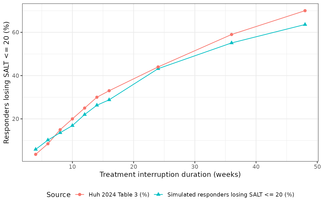
Simulated loss of the SALT <= 20 response after withdrawal of 50 mg QD at week 96, against Huh 2024 Table 3.
Individual profiles across withdrawal, the shape Figure 5B of the paper shows:
solInt %>%
  dplyr::filter(id %in% head(responders, 12)) %>%
  ggplot2::ggplot(ggplot2::aes(x = time, y = salt, group = id)) +
  ggplot2::geom_line(colour = "darkgreen", alpha = 0.8) +
  ggplot2::geom_vline(xintercept = 96, linetype = "dashed", colour = "red") +
  ggplot2::geom_hline(yintercept = 20, linetype = "dotted") +
  ggplot2::labs(x = "Time (weeks)", y = "SALT score") +
  ggplot2::theme_bw()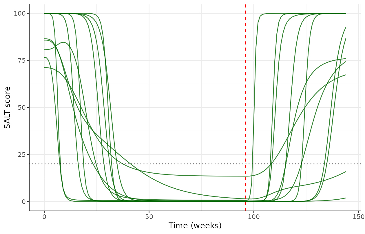
Replicates the shape of Figure 5B of Huh 2024: individual predicted SALT profiles for responders, with treatment withdrawn at week 96 (dashed line).
Replicating Figure 3: dose-response over the simulated dose range
Huh 2024 Figure 3 plots the placebo-adjusted SALT <= 20 responder rate at weeks 24 and 48 for placebo and 30-600 mg QD. Figure 3 is a figure with no tabulated values, so the comparison here is to the claim Section 3.3 makes about it: “higher efficacy is expected at doses greater than 50 mg, with dosages of 400 mg QD approaching the maximum efficacy”.
# Etas come from `cohort`; no rxode2-side sampling is needed.
drDoses <- c(0, 30, 50, 100, 200, 400, 600)
weeksDR <- seq(0, 48, by = 1)

drSolve <- lapply(drDoses, function(d) {
  cav <- if (d == 0) 0 else cavOf(d)
  ev <- makeEvents(data.frame(from = 0, cav = cav), weeksDR, cohort)
  rxode2::rxSolve(pd, ev, omega = NA, sigma = NA,
                  returnType = "data.frame") %>%
    dplyr::mutate(dose = d)
}) %>%
  dplyr::bind_rows()

responderRate <- drSolve %>%
  dplyr::filter(time %in% c(24, 48)) %>%
  dplyr::group_by(dose, time) %>%
  dplyr::summarise(rate = 100 * mean(salt <= 20), .groups = "drop")

pboRate <- responderRate %>%
  dplyr::filter(dose == 0) %>%
  dplyr::select(time, pbo = rate)

adjRate <- responderRate %>%
  dplyr::left_join(pboRate, by = "time") %>%
  dplyr::mutate(adj = rate - pbo) %>%
  dplyr::filter(dose > 0)

adjRate %>%
  dplyr::mutate(Week = paste0("Week ", time)) %>%
  dplyr::select(Week, `Dose (mg QD)` = dose,
                `Placebo-adjusted SALT <= 20 responder rate (%)` = adj) %>%
  dplyr::mutate(`Placebo-adjusted SALT <= 20 responder rate (%)` =
                  round(`Placebo-adjusted SALT <= 20 responder rate (%)`, 1)) %>%
  tidyr::pivot_wider(names_from = Week,
                     values_from = `Placebo-adjusted SALT <= 20 responder rate (%)`) %>%
knitr::kable(caption = "Placebo-adjusted SALT <= 20 responder rate by dose (single simulated trial of 200 participants per arm; Huh 2024 Figure 3 summarises 1000 trials of 130 participants).")| Dose (mg QD) | Week 24 | Week 48 |
|---|---|---|
| 30 | 14.5 | 31.5 |
| 50 | 23.5 | 43.0 |
| 100 | 32.0 | 51.5 |
| 200 | 42.5 | 57.0 |
| 400 | 45.5 | 60.0 |
| 600 | 45.5 | 61.5 |
wk48 <- adjRate %>% dplyr::filter(time == 48) %>% dplyr::arrange(dose)

# The exposure-response relationship must be monotone in dose: the drug term is
# a monotone Emax function of CAV and CAV is monotone in dose.
stopifnot(!is.unsorted(wk48$adj))

# Section 3.3: 400 mg QD approaches maximum efficacy, so the 400 -> 600 mg
# increment must be a small fraction of the 50 -> 400 mg increment.
inc400to600 <- wk48$adj[wk48$dose == 600] - wk48$adj[wk48$dose == 400]
inc50to400  <- wk48$adj[wk48$dose == 400] - wk48$adj[wk48$dose == 50]
cat(sprintf("Week-48 placebo-adjusted responder rate increments: 50 -> 400 mg %.1f points; 400 -> 600 mg %.1f points\n",
            inc50to400, inc400to600))
#> Week-48 placebo-adjusted responder rate increments: 50 -> 400 mg 17.0 points; 400 -> 600 mg 1.5 points
stopifnot(inc50to400 > 0, inc400to600 < 0.35 * inc50to400)
ggplot2::ggplot(adjRate, ggplot2::aes(x = dose, y = adj,
                                      colour = factor(time), shape = factor(time))) +
  ggplot2::geom_line() +
  ggplot2::geom_point(size = 2) +
  ggplot2::scale_x_continuous(breaks = drDoses[drDoses > 0]) +
  ggplot2::labs(x = "Ritlecitinib dose (mg QD)",
                y = "Placebo-adjusted SALT <= 20 responder rate (%)",
                colour = "Week", shape = "Week") +
  ggplot2::theme_bw() +
  ggplot2::theme(legend.position = "bottom")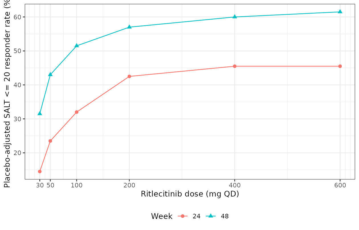
Replicates Figure 3 of Huh 2024: placebo-adjusted SALT <= 20 responder rate at weeks 24 and 48 across the simulated dose range.
Replicating Figure 4: the loading-dose effect
Section 3.4 reports that a 200 mg QD 4-week loading dose brought the clinical onset of the SALT <= 20 response forward by 7 weeks for the 30 mg maintenance group (6 versus 13 weeks) and by 3 weeks for the 50 mg group (6 versus 9 weeks), but that the 95% CIs of the responder rates overlapped at week 48. The paper’s onset definition depends on the 95% CI of 1000 simulated trials, which is out of budget here; the reproducible content is the ordering – loading arms separate earlier and converge by week 48.
# Etas come from `cohort`; no rxode2-side sampling is needed.
weeksLoad <- seq(0, 48, by = 1)
loadArms <- list(
  "30 mg QD"        = data.frame(from = 0,      cav = cavOf(30)),
  "200/30 mg QD"    = data.frame(from = c(0, 4), cav = c(cavOf(200), cavOf(30))),
  "50 mg QD"        = data.frame(from = 0,      cav = cavOf(50)),
  "200/50 mg QD"    = data.frame(from = c(0, 4), cav = c(cavOf(200), cavOf(50))),
  "Placebo"         = data.frame(from = 0,      cav = 0)
)

loadSolve <- lapply(names(loadArms), function(nm) {
  ev <- makeEvents(loadArms[[nm]], weeksLoad, cohort)
  rxode2::rxSolve(pd, ev, omega = NA, sigma = NA,
                  returnType = "data.frame") %>%
    dplyr::mutate(arm = nm)
}) %>%
  dplyr::bind_rows()

loadRate <- loadSolve %>%
  dplyr::group_by(arm, time) %>%
  dplyr::summarise(rate = 100 * mean(salt <= 20), .groups = "drop")

loadPbo <- loadRate %>%
  dplyr::filter(arm == "Placebo") %>%
  dplyr::select(time, pbo = rate)

loadAdj <- loadRate %>%
  dplyr::filter(arm != "Placebo") %>%
  dplyr::left_join(loadPbo, by = "time") %>%
  dplyr::mutate(adj = rate - pbo,
                maintenance = ifelse(grepl("30", arm), "30 mg maintenance",
                                     "50 mg maintenance"),
                loading = ifelse(grepl("^200/", arm), "With 200 mg loading",
                                 "No loading"))
# Onset: the first week at which the placebo-adjusted responder rate exceeds a
# fixed 5-point threshold. This is not the paper's CI-based definition, but it
# ranks the arms the same way.
onset <- loadAdj %>%
  dplyr::filter(adj > 5) %>%
  dplyr::group_by(arm) %>%
  dplyr::summarise(onsetWeek = min(time), .groups = "drop")

onsetTable <- onset %>%
  dplyr::mutate(`Huh 2024 Section 3.4 onset (weeks)` =
                  c(13, 6, 9, 6)[match(arm, c("30 mg QD", "200/30 mg QD",
                                              "50 mg QD", "200/50 mg QD"))]) %>%
  dplyr::rename(Arm = arm, `Simulated onset (weeks)` = onsetWeek)

knitr::kable(onsetTable,
caption = "Onset of the placebo-adjusted SALT <= 20 response. The simulated onset uses a fixed 5-point threshold, not the paper's 95%-CI separation criterion, so only the ordering is comparable.")| Arm | Simulated onset (weeks) | Huh 2024 Section 3.4 onset (weeks) |
|---|---|---|
| 200/30 mg QD | 8 | 6 |
| 200/50 mg QD | 7 | 6 |
| 30 mg QD | 13 | 13 |
| 50 mg QD | 10 | 9 |
wk48load <- loadAdj %>% dplyr::filter(time == 48)

get48 <- function(a) wk48load$adj[wk48load$arm == a]
onsetOf <- function(a) onset$onsetWeek[onset$arm == a]

stopifnot(
  # Despite the different onset criterion, every simulated onset lands within
  # 3 weeks of the paper's, and the 30 mg QD arm matches exactly.
  max(abs(onsetTable$`Simulated onset (weeks)` -
            onsetTable$`Huh 2024 Section 3.4 onset (weeks)`)) <= 3,
  # Loading brings onset forward (or at worst leaves it unchanged) in both
  # maintenance groups -- the paper's central finding for Figure 4.
  onsetOf("200/30 mg QD") <= onsetOf("30 mg QD"),
  onsetOf("200/50 mg QD") <= onsetOf("50 mg QD"),
  # The 30 mg group gains more from loading than the 50 mg group (paper: 7 vs 3
  # weeks), because it sits lower on the ascending exposure-response curve.
  (onsetOf("30 mg QD") - onsetOf("200/30 mg QD")) >=
    (onsetOf("50 mg QD") - onsetOf("200/50 mg QD")),
  # By week 48 the loading and non-loading arms have converged: Section 3.4
  # reports "no long-term benefit".
  abs(get48("200/30 mg QD") - get48("30 mg QD")) < 5,
  abs(get48("200/50 mg QD") - get48("50 mg QD")) < 5
)
ggplot2::ggplot(loadAdj, ggplot2::aes(x = time, y = adj, colour = loading)) +
  ggplot2::geom_line(linewidth = 0.8) +
  ggplot2::facet_wrap(~maintenance) +
  ggplot2::geom_vline(xintercept = 4, linetype = "dashed", colour = "grey40") +
  ggplot2::labs(x = "Time (weeks)",
                y = "Placebo-adjusted SALT <= 20 responder rate (%)",
                colour = NULL) +
  ggplot2::theme_bw() +
  ggplot2::theme(legend.position = "bottom")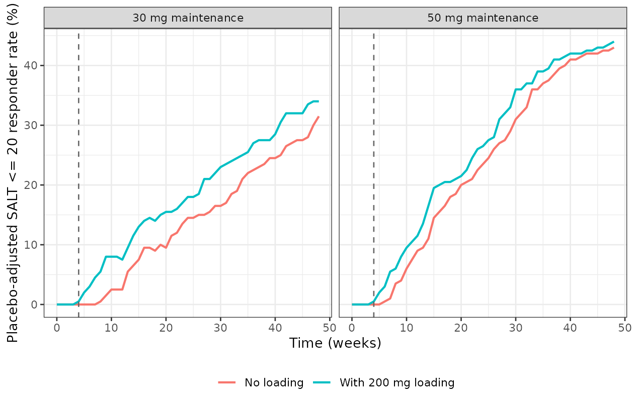
Replicates the efficacy panels of Figure 4 of Huh 2024: placebo-adjusted SALT <= 20 responder rate for loading versus non-loading regimens.
Assumptions and deviations
-
Aranda-Ordaz orientation (Errata). Equation 1 of
the paper, as typeset, defines
z = (100 - y)/100and then applies the transformation to1 - z, which composes toy/100. That composition is falsified twice by the paper’s own numbers. First, Table 2 givesBASEfor the AT/AU group as +11.6 while Section 3.2 states the AT/AU baseline is SALT = 100; under the typeset compositiony -> 100sends the transform to minus infinity, not plus infinity. Second, Section 3.2 states that theEmaxof 15.8 “is translated into a complete recovery in SALT score”, and because Equation 3 subtracts the drug term, that requires the transform to decrease as SALT decreases. Both are satisfied only by applying the transformation to(100 - y)/100, which is what this model encodes. One of the two halves of Equation 1 as printed therefore carries a definition slip; the composite function is unambiguous. -
Baseline back-transforms do not reproduce exactly.
With the published
alpha = 1.19, the inverse transform mapsBASE = 1.92to 84.4% andBASE = 0.68to 63.8%, where Section 3.2 quotes 87.4% and 67.3%. The two parenthetical values are jointly consistent withalphaof about 0.97 rather than 1.19. The AT/AU value (11.6 -> 100%) reproduces exactly. The model uses the printed Table 2 value ofalpha = 1.19; no parameter was tuned to close the gap. -
Maximal-effect SALT for AT/AU does not reproduce.
Section 3.2 quotes 0.33 for the AT/AU group at maximal effect. Under
Equations 1-4 the transformed score at maximal effect is
11.6 - 2.75 - 15.8 = -6.95, which back-transforms to 0.096 for anyalpha(the inverse is approximately100 * exp(x)in this regime, soalphacancels). Recovering 0.33 would require a transformed score of -5.71. The non-AT/AU value reproduces (1.92 - 0 - 15.8 = -13.88-> effectively 0, as the paper states). Both figures are prose illustrations, not model parameters. -
IIV on the drug-chain rate is attached to the
half-life. Table 2 labels the variance row
omega^2 Kout2but labels the covariate row “AT/AU effect on kout2 half-life”, and Section 2.3 states that “t1/2was estimated instead ofkinorkout”. The eta is therefore placed on the half-life, matching the parameter that was estimated and the level the covariate acts on. Placing it on the rate constant instead would flip the sign of its covariance withEmax(Table 2: +0.549). This is the one structural reading in the model that the source does not make explicit. -
IIV on BASE is exponential, not additive. Equation
3’s parenthetical gloss reads “
[BASE + eta]”, but Section 2.3 states explicitly that “IIV was incorporated in BASE, Emax, and kin2/kout2 using a multiplicative exponential error model (Pi = Ppop * exp(eta_i))” and contrasts this withPmax, “with an additive model … to allow both disease worsening and improving”. The Section 2.3 statement is the specific one and is the reading encoded here. -
Pmaxfor the non-AT/AU group is carried asfixed(0)rather than dropped, so the estimated-then-fixed provenance of Table 2’s “0 fix” row survives into the packaged model. - The censored likelihood is not part of the packaged model. Huh 2024 treats SALT records of 0 and 100 as censored when constructing the likelihood (Section 2.3). That is a fitting-time construct; the structural model here approaches the boundaries asymptotically. A user re-fitting this model to bounded SALT data must reinstate the censoring themselves.
-
Fitting requires transformed observations. The
residual error acts on
salt_transformed, so observed SALT scores must be transformed withlog((((100 - SALT)/100)^(-alpha) - 1)/alpha)before being passed to nlmixr2. The back-transformedsaltis emitted alongside for interpretation and plotting. -
CAVis derived here from the packaged PK model at typical values, whereas Huh 2024 used per-subject empirical Bayes estimates of the same PK model combined with each participant’s dosing diary. The 50 mg QD anchor agrees with the paper’s 52 ng/mL, but no per-subject PK variability is propagated into the ER simulations in this vignette. - Random effects are drawn from OMEGA, not from EBEs. The paper’s treatment-interruption and loading-dose simulations used the fitted participants’ empirical Bayes estimates, whose spread is narrowed by the reported 16-37% eta shrinkage. Simulating from the published OMEGA therefore produces a more variable cohort. In practice this costs little: the ten Table 3 proportions are reproduced to within 6.4 percentage points, with the simulated series running slightly high at the shortest interruptions and slightly low at the longest, which is the signature of the wider-than-EBE spread.
- Cohort size. Two hundred participants per arm, against the paper’s 1000 trials of 130 participants (Sections 2.4 and 2.5) and 715 participants (Section 2.6). Single-trial estimates therefore carry sampling noise the paper’s prediction intervals average away.
-
The observation variable is
salt_transformed, notCc.checkModelConventions()emits a non-canonical-observation warning for this, the same warning the packagedWojciechowski_2015_rheumatoidArthritismodel carries. There is no drug-concentration output in this model, soCcdoes not apply. - Supplementary material was not required. Supplementary Table S1 is the SALT assessment schedule, Table S2 the model-development history, and Figures S1-S3 the eta-versus-covariate scatter plots that motivated dropping every covariate. No parameter value used here comes from the supplement.
-
No covariates other than AT/AU status and study were
retained. The nine screened-but-dropped covariates are
preserved in the model’s
covariatesDataExcludedmetadata so the provenance of the covariate screen is not lost.