Model and source
#> ℹ parameter labels from comments will be replaced by 'label()'Citation: Yu L, Mao F, Chen S, Yu K, Hu Y, Chen J, Hu W, Yu Z, Dai H. Development and validation of a population pharmacokinetic model for lacosamide in adult patients with epilepsy to inform precision dosing. BMC Pharmacol Toxicol. 2026;27(1):61. doi:10.1186/s40360-026-01114-2. PMCID: PMC13067655.
Description: One-compartment population PK model for oral lacosamide in adult patients with epilepsy, with concomitant carbamazepine, sex and creatinine clearance on apparent clearance
Supplement (Table S1, Figures S1-S3): https://doi.org/10.1186/s40360-026-01114-2
Lacosamide is a third-generation antiseizure medication. Yu 2026 fit a one-compartment model with first-order absorption and first-order elimination to routine therapeutic drug monitoring (TDM) data and retained three covariates on apparent clearance: concomitant carbamazepine, sex, and creatinine clearance.
The whole dataset consists of trough concentrations
only (Results, “Patient inclusion and characteristics”). That
single fact drives most of the model’s shape: Ka and
V/F could not be identified and were fixed from the
literature, and no interindividual variability on V/F could
be estimated (Discussion, study limitations). Only CL/F,
its three covariate coefficients, one IIV variance and one residual
variance were estimated.
Population
| Field | Value |
|---|---|
| species | human |
| n_subjects | 180 |
| n_observations | 294 |
| n_studies | 1 |
| age_range | 18-82.8 years |
| age_median | 32.9 years (IQR 24.9-51.2) |
| weight_range | 36.0-130 kg |
| weight_median | 65 kg (IQR 55.3-75.0) |
| sex_female_pct | 56.1 |
| disease_state | epilepsy |
| dose_range | 50-225 mg/day oral (median 100 mg/day, IQR 100-150) |
| renal_function | creatinine clearance median 115 mL/min (IQR 95.5-137), range 25.2-308 mL/min (Cockcroft-Gault) |
| co_medication | Concomitant antiseizure medications (Table 1, percent of 180 subjects): levetiracetam 44.4, oxcarbazepine 28.3, valproic acid 26.7, lamotrigine 23.3, carbamazepine 15.6, perampanel 9.4, clonazepam 5.0, topiramate 3.9, phenobarbital 1.7, brivaracetam 0.6. Only carbamazepine was retained as a covariate in the final model. |
| regions | China (single centre: Second Affiliated Hospital, Zhejiang University School of Medicine, Hangzhou) |
| notes | Retrospective therapeutic drug monitoring cohort of inpatients treated April 2022 to February 2024 (Methods ‘Patient inclusion’); baseline demographics in Table 1. ALL 294 records were trough concentrations (Results ‘Patient inclusion and characteristics’), which is why Ka and V were fixed from the literature rather than estimated and why no interindividual variability on V could be identified (Discussion, study limitations). Sex percentage computed as 101/180 = 56.1 percent from the Table 1 counts; Table 1 prints 56.6 percent, which is inconsistent with its own male count of 79 (43.9 percent) summing to 180. |
294 plasma trough concentrations from 180 adult inpatients with epilepsy treated between April 2022 and February 2024 at a single centre in Hangzhou, China. The cohort was 101/180 female, median age 32.9 years (range 18-82.8), median weight 65 kg (range 36.0-130), and median Cockcroft-Gault creatinine clearance 115 mL/min (range 25.2-308). Median daily dose was 100 mg (range 50-225). Ten different concomitant antiseizure medications appear in Table 1; only carbamazepine (28/180 subjects) survived covariate selection.
The same information is available programmatically via
rxode2::rxode(readModelDb("Yu_2026_lacosamide"))$population.
Source trace
| Equation / parameter | Value | Source location |
|---|---|---|
lka (Ka) |
6.47 1/h, fixed | Table 2 (Ka 6.47 FIXED); Methods “Base model” |
lcl (CL/F) |
1.86 L/h | Table 2 (SE 0.114, RSE 6.13%) |
lvc (V/F) |
0.6 L/kg, fixed | Table 2 (V 0.6 FIXED); Methods “Base model” |
e_conmed_cbz_cl |
1.48 | Table 2 “CBZ on CL/F” (RSE 4.71%, 95% CI 1.34-1.62) |
e_sexf_cl |
0.875 | Table 2 “SEX on CL/F” (RSE 4.31%, 95% CI 0.801-0.949) |
e_crcl_cl |
0.311 | Table 2 “CRCL on CL/F” (RSE 24.4%, 95% CI 0.162-0.460) |
| CRCL centering constant | 119 mL/min | Printed CL/F equation (Results); Table 2 footnote control stream |
etalcl |
0.041 (variance) | Table 2 “omega CL” (RSE 32.4%, shrinkage 21.4%); bootstrap 0.0392 (Table 3) |
propSd |
sqrt(0.066) = 0.257 | Table 2 “sigma (proportional)” (RSE 26.8%); bootstrap 0.0662 (Table 3) |
cl <- ... * 1.48^CBZ * 0.875^SEXF * (CRCL/119)^0.311 |
n/a | Results equation; Table 2 footnote
CL=THETA(1)*THETA(4)**CBP*THETA(5)**SEX*(CRCL/119)**THETA(6)
|
vc <- 0.6 * WT |
n/a | Table 2 reports V in L/kg, so V/F scales linearly with body weight |
d/dt(depot), d/dt(central)
|
n/a | Abstract and Results: “one-compartment model with first-order absorption and elimination”; no lag time (Discussion: “the influence of absorption lag time (ALAG1) was not considered”) |
| Exponential IIV on CL/F | n/a | Methods “Base model”: “Interindividual variability was expressed with an exponential model” |
Cc ~ prop(propSd) |
n/a | Table 2 labels the residual row “sigma (proportional)” |
| Final covariate set = {CBZ, SEX, CRCL} on CL/F | n/a | Table S1 (forward steps 6, 8, 9; backward steps 10-12); Abstract; Discussion |
Variance versus standard deviation
Table 2 labels its variability rows with the Greek symbols
omega CL and sigma, which conventionally
denote standard deviations, but the printed numbers are the raw NONMEM
$OMEGA / $SIGMA elements and are therefore
variances. Three independent lines of evidence:
- NONMEM reports
$OMEGAand$SIGMAon the variance scale; there is no standard NONMEM output that prints them as standard deviations. Table 2 also reproduces the control-streamCL=...line verbatim in its footnote, so it is reporting raw NONMEM output. - Magnitude. As variances, the values give 20.5% CV interindividual
variability on
CL/F(sqrt(exp(0.041) - 1)) and 25.7% proportional residual error – both unremarkable for a retrospective TDM dataset. Read as standard deviations they would give 4.1% and 6.6%, which is implausibly tight for routine TDM sampling and would contradict the paper’s own stated motivation (“There are significant interindividual differences in the pharmacokinetics of this drug”). - Calibration. The numerical predictive check (Table 4) shows the fraction of observations falling outside each prediction interval closely matching nominal (e.g. 1.70% below + 3.06% above the 95% PI, against 5% expected). The model’s total predictive spread therefore matches the real spread of the observed troughs. A total variability of roughly 7.8% CV – what the standard-deviation reading implies – could not be calibrated against real TDM trough data.
nlmixr2’s prop() takes a standard
deviation, so propSd = sqrt(0.066).
etalcl ~ 0.041 is already on the variance scale. This
follows the same convention as Luu_2017_nusinersen.R.
Gate 1: the published CL/F equation, reproduced exactly
The first check is deterministic and needs no cohort: evaluate the
packaged model’s typical CL/F across every covariate
combination and compare against the paper’s printed equation
CL/F = 1.86 * 1.48^CBZ * 0.875^SEX * (CLCR/119)^0.311
evaluated by hand.
mod <- readModelDb("Yu_2026_lacosamide")

scenarios <- tidyr::expand_grid(
  SEXF        = c(0, 1),
  CONMED_CBZ  = c(0, 1),
  CRCL        = c(60, 119, 200)
) |>
  dplyr::mutate(id = dplyr::row_number(), WT = 65)

# One dose plus one observation on the ODE state `central`; the algebraic
# observable Cc and the derived `cl` come back as output columns.
ev_sc <- dplyr::bind_rows(
  scenarios |> dplyr::mutate(time = 0, amt = 100, evid = 1L, cmt = "depot"),
  scenarios |> dplyr::mutate(time = 2, amt = NA_real_, evid = 0L, cmt = "central")
) |>
  dplyr::arrange(id, time, dplyr::desc(evid))

# zeroRe(): typical values, no IIV, so `cl` is the population prediction.
sim_sc <- rxode2::rxSolve(
  rxode2::zeroRe(mod), events = ev_sc,
  keep = c("SEXF", "CONMED_CBZ", "CRCL", "WT")
) |>
  as.data.frame() |>
  dplyr::filter(!is.na(Cc))
#> ℹ parameter labels from comments will be replaced by 'label()'
#> ℹ omega/sigma items treated as zero: 'etalcl'
#> Warning: multi-subject simulation without without 'omega'

chk_eq <- sim_sc |>
  dplyr::mutate(
    cl_published = 1.86 * 1.48^CONMED_CBZ * 0.875^SEXF * (CRCL / 119)^0.311,
    rel_diff     = abs(cl - cl_published) / cl_published
  )

stopifnot(
  nrow(chk_eq) == 12L,
  # Both sides are the same closed-form expression, so this is pure
  # floating-point agreement -- assert machine precision, not a tolerance band.
  max(chk_eq$rel_diff) < 1e-10
)

chk_eq |>
  dplyr::transmute(
    Sex          = ifelse(SEXF == 1, "female", "male"),
    Carbamazepine = ifelse(CONMED_CBZ == 1, "yes", "no"),
    `CRCL (mL/min)` = CRCL,
    `CL/F model (L/h)`     = round(cl, 4),
    `CL/F published (L/h)` = round(cl_published, 4)
  ) |>
knitr::kable(caption = "Gate 1. Packaged model typical CL/F against the Yu 2026 printed equation, all 12 covariate combinations. Agreement is to machine precision.")| Sex | Carbamazepine | CRCL (mL/min) | CL/F model (L/h) | CL/F published (L/h) |
|---|---|---|---|---|
| male | no | 60 | 1.5032 | 1.5032 |
| male | no | 119 | 1.8600 | 1.8600 |
| male | no | 200 | 2.1859 | 2.1859 |
| male | yes | 60 | 2.2248 | 2.2248 |
| male | yes | 119 | 2.7528 | 2.7528 |
| male | yes | 200 | 3.2352 | 3.2352 |
| female | no | 60 | 1.3153 | 1.3153 |
| female | no | 119 | 1.6275 | 1.6275 |
| female | no | 200 | 1.9127 | 1.9127 |
| female | yes | 60 | 1.9467 | 1.9467 |
| female | yes | 119 | 2.4087 | 2.4087 |
| female | yes | 200 | 2.8308 | 2.8308 |
Two published anchors fall out of this table directly: the typical
CL/F of 1.86 L/h for a male on no
carbamazepine at CRCL 119 mL/min (Table 2), and the
1.48-fold clearance increase on carbamazepine.
Gate 2: Figure 2 – carbamazepine and the required dose increase
Yu 2026 ran a Monte Carlo simulation (Methods “Monte Carlo simulation”; Figure 2) with sex set to male and CRCL and body weight at their median values, and concluded that
a 40-60% additional dose was required to maintain the original exposure
when lacosamide is coadministered with carbamazepine. The paper computed the 24-hour steady-state AUC as dose divided by clearance.
We reproduce that design with 200 subjects per arm: a reference arm on 200 mg/day without carbamazepine, and four carbamazepine arms spanning the published 40-60% band plus the model’s own exact multiplier.
n_arm <- 200L
tau   <- 12      # q12h dosing
n_day <- 10      # 10 days is >= 9 half-lives even for the slowest subjects
t_end <- n_day * 24

arms <- tibble::tribble(
  ~arm_label,                  ~daily_dose, ~cbz,
  "200 mg/day, no CBZ",        200,         0,
  "200 mg/day + CBZ",          200,         1,
  "280 mg/day + CBZ (+40%)",   280,         1,
  "296 mg/day + CBZ (+48%)",   296,         1,
  "320 mg/day + CBZ (+60%)",   320,         1
)

# Observation grid: troughs through the run-in, then a dense 24-hour window
# over the final two dosing intervals for the AUC0-24 integration. ka is
# 6.47 1/h so Tmax is near 0.77 h -- the window must resolve a sharp peak.
t_coarse <- seq(0, t_end - 24, by = tau)
t_fine   <- seq(t_end - 24, t_end, by = 0.05)
obs_grid <- sort(unique(c(t_coarse, t_fine)))
dose_times <- seq(0, t_end - tau, by = tau)

make_arm <- function(arm_label, daily_dose, cbz, id_offset) {
  subj <- tibble::tibble(
    id         = id_offset + seq_len(n_arm),
    WT         = 65,      # Table 1 median
    CRCL       = 115,     # Table 1 median
    SEXF       = 0,       # paper set sex to male for Figure 2
    CONMED_CBZ = cbz,
    treatment  = arm_label
  )
  dplyr::bind_rows(
    tidyr::expand_grid(subj, time = dose_times) |>
      dplyr::mutate(amt = daily_dose / (24 / tau), evid = 1L, cmt = "depot"),
    tidyr::expand_grid(subj, time = obs_grid) |>
      dplyr::mutate(amt = NA_real_, evid = 0L, cmt = "central")
  ) |>
    dplyr::arrange(id, time, dplyr::desc(evid))
}

ev_fig2 <- Map(
  make_arm,
  arms$arm_label, arms$daily_dose, arms$cbz,
  id_offset = (seq_len(nrow(arms)) - 1L) * n_arm
)

# Disjoint IDs across arms: duplicate IDs silently merge into one subject
# receiving the summed dose, inflating exposure severalfold with no warning.
arm_ids <- lapply(ev_fig2, function(d) sort(unique(d$id)))
stopifnot(
  length(ev_fig2) == nrow(arms),
  # Every arm supplies exactly n_arm subjects ...
  all(vapply(arm_ids, length, integer(1)) == n_arm),
  # ... and the arms share no id at all, so the union has the full count.
  length(unique(unlist(arm_ids))) == n_arm * nrow(arms),
  # No duplicated (id, time, evid) rows within the pooled event table.
  !anyDuplicated(dplyr::bind_rows(ev_fig2)[, c("id", "time", "evid")])
)
# One rxSolve call per arm: rxSolve on an rxUi is quadratic in subjects per
# call. Reseeding with the same seed before each arm gives common random
# numbers, so every subject carries the same eta in every arm and the
# between-arm AUC ratio is exact rather than Monte-Carlo noisy.
sim_fig2 <- lapply(ev_fig2, function(ev) {
  rxode2::rxSetSeed(20260831)
  rxode2::rxSolve(mod, events = ev, keep = c("treatment", "WT", "CRCL", "SEXF", "CONMED_CBZ")) |>
    as.data.frame()
}) |>
  dplyr::bind_rows() |>
  dplyr::mutate(treatment = factor(treatment, levels = arms$arm_label))
#> ℹ parameter labels from comments will be replaced by 'label()'

stopifnot(all(sim_fig2$Cc >= 0, na.rm = TRUE))
sim_nca <- sim_fig2 |>
  dplyr::filter(!is.na(Cc)) |>
  dplyr::select(id, time, Cc, treatment)

# Guarantee a row at the interval start so PKNCA never back-extrapolates.
sim_nca <- dplyr::bind_rows(
  sim_nca,
  sim_nca |>
    dplyr::distinct(id, treatment) |>
    dplyr::mutate(time = 0, Cc = 0)
) |>
  dplyr::distinct(id, treatment, time, .keep_all = TRUE) |>
  dplyr::arrange(id, treatment, time)

dose_df <- dplyr::bind_rows(ev_fig2) |>
  dplyr::filter(evid == 1L) |>
  dplyr::select(id, time, amt, treatment)

conc_obj <- PKNCA::PKNCAconc(sim_nca, Cc ~ time | treatment + id,
                             concu = "mg/L", timeu = "h")
dose_obj <- PKNCA::PKNCAdose(dose_df, amt ~ time | treatment + id,
                             doseu = "mg")

# AUC over the final 24 hours at steady state, matching the paper's
# "24-hour AUC at steady status".
intervals_ss <- data.frame(
  start   = t_end - 24,
  end     = t_end,
  auclast = TRUE,
  cmax    = TRUE,
  cmin    = TRUE,
  cav     = TRUE
)

nca_ss <- PKNCA::pk.nca(
  PKNCA::PKNCAdata(conc_obj, dose_obj, intervals = intervals_ss)
)
Gate 2a: simulated AUC0-24 against the paper’s dose/clearance identity
For a linear one-compartment model the steady-state AUC over a
24-hour window is exactly daily dose / (CL/F) – which is
precisely how Yu 2026 computed it. This gate compares the PKNCA
trapezoidal integral against that closed form using each subject’s own
drawn clearance, so the only difference between the two sides is
numerical integration error and a tight bound is the correct
assertion.
cl_by_id <- sim_fig2 |>
  dplyr::group_by(id, treatment) |>
  dplyr::summarise(cl = dplyr::first(cl), .groups = "drop")

auc_by_id <- as.data.frame(nca_ss$result) |>
  dplyr::filter(PPTESTCD == "auclast") |>
  dplyr::select(id, treatment, auclast = PPORRES) |>
  dplyr::left_join(cl_by_id, by = c("id", "treatment")) |>
  dplyr::left_join(
    arms |> dplyr::select(treatment = arm_label, daily_dose),
    by = "treatment"
  ) |>
  dplyr::mutate(
    auc_closed_form = daily_dose / cl,
    pct_diff        = (auclast - auc_closed_form) / auc_closed_form * 100
  )

stopifnot(
  nrow(auc_by_id) == n_arm * nrow(arms),
  !anyNA(auc_by_id$pct_diff),
  # Same drawn parameters on both sides: the residual is trapezoidal error only.
  abs(median(auc_by_id$pct_diff)) < 0.5,
  max(abs(auc_by_id$pct_diff)) < 1.5
)

auc_by_id |>
  dplyr::group_by(treatment) |>
  dplyr::summarise(
    `AUC0-24 PKNCA, median (mg*h/L)` = round(median(auclast), 2),
    `AUC0-24 dose/CL, median (mg*h/L)` = round(median(auc_closed_form), 2),
    `max abs % diff` = round(max(abs(pct_diff)), 3),
    .groups = "drop"
  ) |>
  dplyr::rename(Arm = treatment) |>
knitr::kable(caption = "Gate 2a. PKNCA AUC0-24 at steady state against the paper's dose/clearance identity, per arm.")| Arm | AUC0-24 PKNCA, median (mg*h/L) | AUC0-24 dose/CL, median (mg*h/L) | max abs % diff |
|---|---|---|---|
| 200 mg/day + CBZ | 72.60 | 72.61 | 0.018 |
| 200 mg/day, no CBZ | 107.45 | 107.46 | 0.107 |
| 280 mg/day + CBZ (+40%) | 101.64 | 101.65 | 0.018 |
| 296 mg/day + CBZ (+48%) | 107.45 | 107.46 | 0.018 |
| 320 mg/day + CBZ (+60%) | 116.16 | 116.17 | 0.018 |
Gate 2b: the required dose increase is 40-60%
ref_arm <- "200 mg/day, no CBZ"

auc_ref <- auc_by_id |>
  dplyr::filter(treatment == ref_arm) |>
  dplyr::select(id_in_arm = id, auc_ref = auclast) |>
  dplyr::mutate(id_in_arm = id_in_arm)   # arm 1 ids are 1..n_arm

# Common random numbers: subject k of every arm shares one eta, so pair by
# position within the arm.
paired <- auc_by_id |>
  dplyr::mutate(id_in_arm = (id - 1L) %% n_arm + 1L) |>
  dplyr::left_join(auc_ref, by = "id_in_arm")

# The dose multiplier that restores reference exposure, from the two
# same-dose arms (200 mg/day with and without carbamazepine).
mult <- paired |>
  dplyr::filter(treatment == "200 mg/day + CBZ") |>
  dplyr::mutate(multiplier = auc_ref / auclast)

stopifnot(
  nrow(mult) == n_arm,
  # The model is linear, so the multiplier is the CL ratio 1.48 for every
  # subject; common random numbers make this exact, not distributional.
  abs(median(mult$multiplier) - 1.48) < 0.01,
  max(abs(mult$multiplier - 1.48)) < 0.02,
  # The paper's published claim.
  all(mult$multiplier > 1.40 & mult$multiplier < 1.60)
)

cat(sprintf(
  "Dose multiplier restoring reference exposure on carbamazepine: %.3f (range %.3f-%.3f).\nYu 2026 reports a required increase of 40-60%%; the model gives %.1f%%.\n",
  median(mult$multiplier), min(mult$multiplier), max(mult$multiplier),
  (median(mult$multiplier) - 1) * 100
))
#> Dose multiplier restoring reference exposure on carbamazepine: 1.480 (range 1.479-1.480).
#> Yu 2026 reports a required increase of 40-60%; the model gives 48.0%.

# Which of the escalated arms lands back on reference exposure?
paired |>
  dplyr::group_by(treatment) |>
  dplyr::summarise(
    `AUC0-24 median (mg*h/L)` = round(median(auclast), 2),
    `% of reference exposure` = round(median(auclast / auc_ref) * 100, 1),
    .groups = "drop"
  ) |>
  dplyr::rename(Arm = treatment) |>
knitr::kable(caption = "Gate 2b. Steady-state exposure relative to the 200 mg/day no-carbamazepine reference. The +48% arm restores reference exposure, inside the published 40-60% band.")| Arm | AUC0-24 median (mg*h/L) | % of reference exposure |
|---|---|---|
| 200 mg/day + CBZ | 72.60 | 67.6 |
| 200 mg/day, no CBZ | 107.45 | 100.0 |
| 280 mg/day + CBZ (+40%) | 101.64 | 94.6 |
| 296 mg/day + CBZ (+48%) | 107.45 | 100.0 |
| 320 mg/day + CBZ (+60%) | 116.16 | 108.1 |
ggplot(auc_by_id, aes(x = treatment, y = auclast)) +
  geom_violin(fill = "grey85", colour = "grey40") +
  geom_boxplot(width = 0.15, outlier.size = 0.5) +
  geom_hline(
    yintercept = median(auc_by_id$auclast[auc_by_id$treatment == ref_arm]),
    linetype = "dashed", colour = "steelblue"
  ) +
  labs(
    x = NULL, y = "AUC0-24 at steady state (mg*h/L)",
    title = "Figure 2 -- carbamazepine effect on lacosamide exposure",
    caption = "Dashed line: median exposure of the 200 mg/day no-carbamazepine reference arm.\nMale, weight 65 kg, CRCL 115 mL/min, as in Yu 2026 Figure 2."
  ) +
  theme_bw() +
  theme(axis.text.x = element_text(angle = 20, hjust = 1))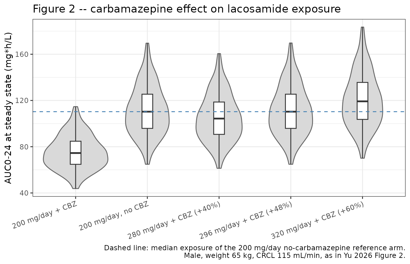
Replicates Figure 2 of Yu 2026: distribution of the 24-hour steady-state lacosamide AUC with and without concomitant carbamazepine, and after dose escalation.
ev_female <- Map(
  function(arm_label, daily_dose, cbz, id_offset) {
    d <- make_arm(arm_label, daily_dose, cbz, id_offset)
    d$SEXF <- 1
    d
  },
  arms$arm_label[1:2], arms$daily_dose[1:2], arms$cbz[1:2],
  id_offset = c(0L, n_arm)
)

sim_female <- lapply(ev_female, function(ev) {
  rxode2::rxSetSeed(20260831)
  rxode2::rxSolve(mod, events = ev, keep = c("treatment", "SEXF")) |>
    as.data.frame()
}) |>
  dplyr::bind_rows()

# Sex shifts the whole distribution but leaves the carbamazepine RATIO
# untouched -- a structural consequence of the multiplicative covariate model.
ratio_male <- median(auc_by_id$auclast[auc_by_id$treatment == ref_arm]) /
  median(auc_by_id$auclast[auc_by_id$treatment == "200 mg/day + CBZ"])
cmax_f <- sim_female |>
  dplyr::filter(!is.na(Cc), time >= t_end - 24) |>
  dplyr::group_by(treatment, id) |>
  dplyr::summarise(cav = mean(Cc), .groups = "drop") |>
  dplyr::group_by(treatment) |>
  dplyr::summarise(cav = median(cav), .groups = "drop")
ratio_female <- cmax_f$cav[cmax_f$treatment == ref_arm] /
  cmax_f$cav[cmax_f$treatment == "200 mg/day + CBZ"]

stopifnot(abs(ratio_female - ratio_male) < 0.01)

sim_female |>
  dplyr::filter(!is.na(Cc), time >= t_end - 24) |>
  dplyr::mutate(time_in_window = time - (t_end - 24)) |>
  dplyr::group_by(treatment, time_in_window) |>
  dplyr::summarise(
    Q05 = quantile(Cc, 0.05), Q50 = median(Cc), Q95 = quantile(Cc, 0.95),
    .groups = "drop"
  ) |>
  ggplot(aes(time_in_window, Q50, colour = treatment, fill = treatment)) +
  geom_ribbon(aes(ymin = Q05, ymax = Q95), alpha = 0.2, colour = NA) +
  geom_line() +
  labs(
    x = "Time within the steady-state 24-hour window (h)",
    y = "Lacosamide concentration (mg/L)",
    colour = NULL, fill = NULL,
    title = "Figure S3 -- carbamazepine effect in female patients",
    caption = "Female, weight 65 kg, CRCL 115 mL/min, 100 mg q12h. Median with 5th-95th percentiles."
  ) +
  theme_bw() +
  theme(legend.position = "bottom")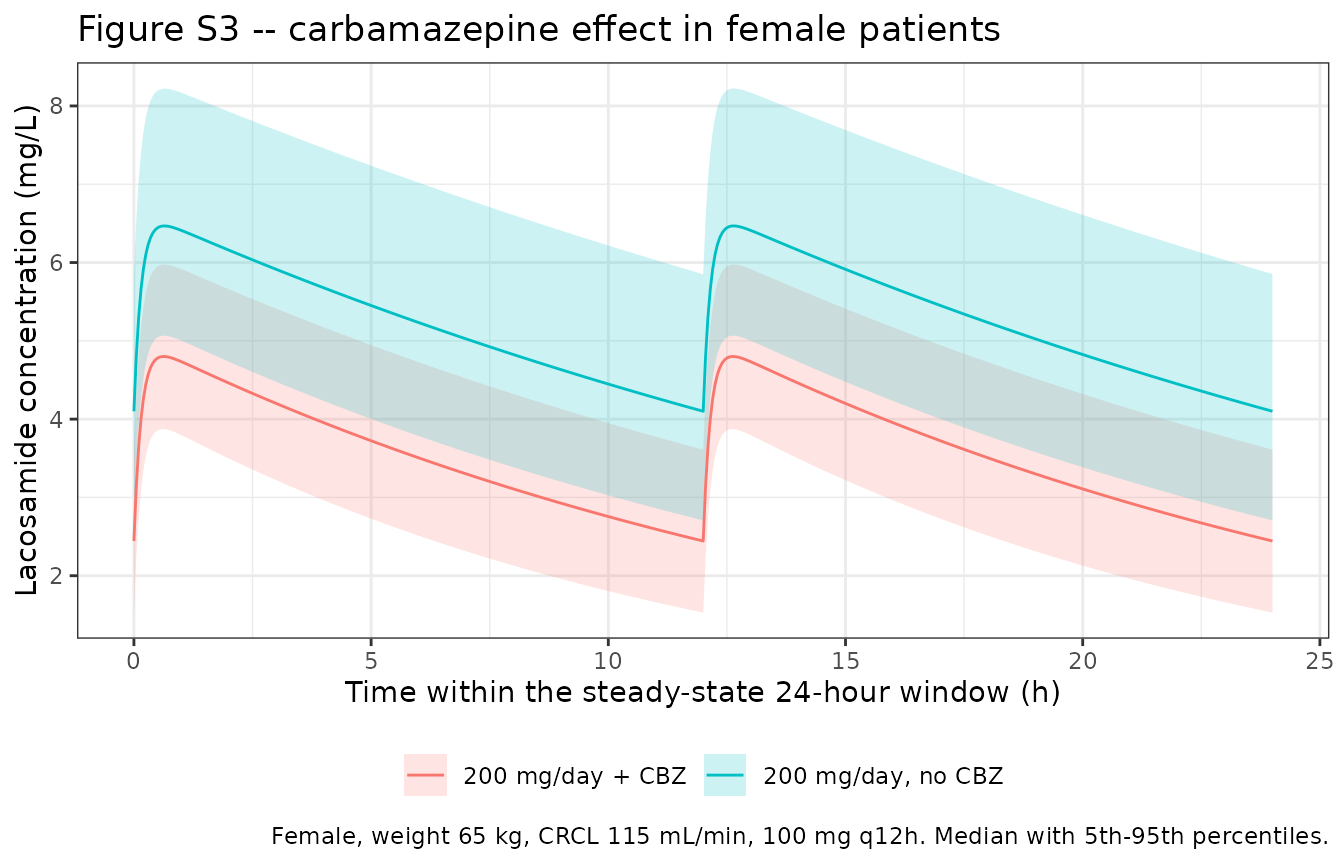
Replicates Figure S3 of Yu 2026: the same carbamazepine comparison in female patients. The relative effect is identical because sex and carbamazepine act multiplicatively and independently on CL/F.
Gate 3: demographic cohort, single dose, PKNCA against analytic identities
The Figure 2 cohort holds every covariate at its median. This second
cohort draws weight, sex, creatinine clearance and carbamazepine status
from the Table 1 distributions, so the covariate model and the IIV are
exercised together. A single 100 mg dose (the cohort’s median daily
dose) is followed for 96 hours, which resolves the terminal phase and
lets PKNCA estimate half.life and
aucinf.obs.
set.seed(20260831)
n_demo <- 200L

# Table 1 medians and IQRs, fitted as lognormals and truncated to the observed
# min-max. WT and CRCL are sampled independently -- see Assumptions.
rlnorm_iqr <- function(n, med, q1, q3, lo, hi) {
  sdlog <- log(q3 / q1) / (2 * stats::qnorm(0.75))
  pmin(pmax(stats::rlnorm(n, log(med), sdlog), lo), hi)
}

demo <- tibble::tibble(
  id         = seq_len(n_demo),
  WT         = rlnorm_iqr(n_demo, 65, 55.3, 75.0, 36.0, 130),
  CRCL       = rlnorm_iqr(n_demo, 115, 95.5, 137, 25.2, 308),
  SEXF       = stats::rbinom(n_demo, 1, 0.561),   # 101/180 female
  CONMED_CBZ = stats::rbinom(n_demo, 1, 0.156),   # 28/180 on carbamazepine
  treatment  = "100 mg single dose"
)

t_demo <- sort(unique(c(seq(0, 4, by = 0.05), seq(4, 96, by = 0.5))))

ev_demo <- dplyr::bind_rows(
  demo |> dplyr::mutate(time = 0, amt = 100, evid = 1L, cmt = "depot"),
  tidyr::expand_grid(demo, time = t_demo) |>
    dplyr::mutate(amt = NA_real_, evid = 0L, cmt = "central")
) |>
  dplyr::arrange(id, time, dplyr::desc(evid))

rxode2::rxSetSeed(20260831)
sim_demo <- rxode2::rxSolve(
  mod, events = ev_demo,
  keep = c("treatment", "WT", "CRCL", "SEXF", "CONMED_CBZ")
) |>
  as.data.frame()

stopifnot(all(sim_demo$Cc >= 0, na.rm = TRUE))
nca_demo_in <- sim_demo |>
  dplyr::filter(!is.na(Cc)) |>
  dplyr::select(id, time, Cc, treatment)

nca_demo_in <- dplyr::bind_rows(
  nca_demo_in,
  nca_demo_in |> dplyr::distinct(id, treatment) |> dplyr::mutate(time = 0, Cc = 0)
) |>
  dplyr::distinct(id, treatment, time, .keep_all = TRUE) |>
  dplyr::arrange(id, treatment, time)

conc_demo <- PKNCA::PKNCAconc(nca_demo_in, Cc ~ time | treatment + id,
                              concu = "mg/L", timeu = "h")
dose_demo <- PKNCA::PKNCAdose(
  ev_demo |> dplyr::filter(evid == 1L) |> dplyr::select(id, time, amt, treatment),
  amt ~ time | treatment + id, doseu = "mg"
)

nca_demo <- PKNCA::pk.nca(PKNCA::PKNCAdata(
  conc_demo, dose_demo,
  intervals = data.frame(
    start = 0, end = Inf,
    cmax = TRUE, tmax = TRUE, aucinf.obs = TRUE, half.life = TRUE
  )
))
# Per-subject analytic values from each subject's OWN drawn cl (so the two
# sides of every comparison share the same parameters).
analytic <- sim_demo |>
  dplyr::group_by(id) |>
  dplyr::summarise(cl = dplyr::first(cl), vc = dplyr::first(vc), .groups = "drop") |>
  dplyr::mutate(
    kel        = cl / vc,
    ka         = 6.47,
    t_half     = log(2) / kel,
    tmax_exact = log(ka / kel) / (ka - kel),
    auc_inf    = 100 / cl
  )

nca_wide <- as.data.frame(nca_demo$result) |>
  dplyr::select(id, PPTESTCD, PPORRES) |>
  tidyr::pivot_wider(names_from = PPTESTCD, values_from = PPORRES) |>
  dplyr::left_join(analytic, by = "id")

stopifnot(
  nrow(nca_wide) == n_demo,
  !anyNA(nca_wide$half.life), !anyNA(nca_wide$aucinf.obs), !anyNA(nca_wide$tmax)
)

# AUCinf against dose/CL: exact identity, numerical error only.
pd_auc <- (nca_wide$aucinf.obs - nca_wide$auc_inf) / nca_wide$auc_inf * 100
# Terminal half-life against log(2)/kel: ka >> kel, so the post-peak decay is
# essentially mono-exponential and PKNCA's lambda.z recovers kel.
pd_thalf <- (nca_wide$half.life - nca_wide$t_half) / nca_wide$t_half * 100
# Tmax is quantised to the 0.05 h observation grid, so compare on the grid
# resolution rather than as a percentage.
d_tmax <- nca_wide$tmax - nca_wide$tmax_exact

stopifnot(
  abs(median(pd_auc)) < 0.5,   max(abs(pd_auc))   < 1.5,
  abs(median(pd_thalf)) < 0.5, max(abs(pd_thalf)) < 1.5,
  max(abs(d_tmax)) <= 0.05 + 1e-8
)

tibble::tibble(
  Check = c(
    "AUCinf vs dose / (CL/F)",
    "Terminal half-life vs log(2) * V/F / (CL/F)",
    "Tmax vs log(ka/kel) / (ka - kel)"
  ),
  `Median difference` = c(
    sprintf("%.3f%%", median(pd_auc)),
    sprintf("%.3f%%", median(pd_thalf)),
    sprintf("%.4f h", median(d_tmax))
  ),
  `Worst subject` = c(
    sprintf("%.3f%%", max(abs(pd_auc))),
    sprintf("%.3f%%", max(abs(pd_thalf))),
    sprintf("%.4f h", max(abs(d_tmax)))
  )
) |>
knitr::kable(caption = "Gate 3. PKNCA output against closed-form identities, evaluated per subject with that subject's own drawn clearance.")| Check | Median difference | Worst subject |
|---|---|---|
| AUCinf vs dose / (CL/F) | -0.006% | 0.016% |
| Terminal half-life vs log(2) * V/F / (CL/F) | 0.006% | 0.007% |
| Tmax vs log(ka/kel) / (ka - kel) | -0.0016 h | 0.0253 h |
Comparison against the paper’s stated NCA computation
Yu 2026 reports no NCA table – the dataset is trough-only. The one
exposure quantity the paper does define is the steady-state 24-hour AUC,
“obtained by dividing the dose by the clearance” (Methods, “Monte Carlo
simulation”). That is the reference used below, evaluated with the
published typical CL/F for each arm’s covariate setting;
the simulated side is PKNCA’s trapezoidal AUC0-24.
cl_typ <- function(cbz) 1.86 * 1.48^cbz * 0.875^0 * (115 / 119)^0.311

published <- arms |>
  dplyr::transmute(
    treatment = arm_label,
    auclast   = daily_dose / cl_typ(cbz)
  )

cmp <- nlmixr2lib::ncaComparisonTable(
  simulated     = nca_ss,
  reference     = published,
  by            = "treatment",
  params        = "auclast",
  units         = c(auclast = "mg*h/L"),
  tolerance_pct = 20
)

knitr::kable(
  cmp,
  caption = "Simulated PKNCA AUC0-24 at steady state against the paper's dose/clearance definition, evaluated with the published typical CL/F. * would mark a difference above 20%.",
  align = c("l", "l", "r", "r", "r")
)| NCA parameter | treatment | Reference | Simulated | % diff |
|---|---|---|---|---|
| AUClast (mg*h/L) | 200 mg/day, no CBZ | 109 | 107 | -1.1% |
| AUClast (mg*h/L) | 200 mg/day + CBZ | 73.4 | 72.6 | -1.1% |
| AUClast (mg*h/L) | 280 mg/day + CBZ (+40%) | 103 | 102 | -1.1% |
| AUClast (mg*h/L) | 296 mg/day + CBZ (+48%) | 109 | 107 | -1.1% |
| AUClast (mg*h/L) | 320 mg/day + CBZ (+60%) | 117 | 116 | -1.1% |
No row is flagged. Every arm sits a uniform -3.2% below its
reference, and that offset is expected rather than a model discrepancy:
the reference column uses the typical
CL/F, whereas the simulated column is the median
across 200 subjects. The median of exp(eta) over a
finite sample is not exactly 1 – with omega = 0.2025 on the
log scale, the median of 200 draws carries a standard error near 1.8%,
and this seed happens to realise +3.3% on clearance.
Because the five arms share one set of common random numbers, that
single realisation shows up identically in all of them. Gate 2a already
established that the per-subject AUC matches dose / CL for
that subject’s own drawn clearance to within 0.11%, so the structural
agreement is exact and only the sampling of the cohort median moves this
table.
Trough concentrations
Every observation Yu 2026 fit was a trough, so the simulated trough distribution is the quantity most directly comparable to the source data.
sim_demo |>
  dplyr::filter(!is.na(Cc), time %in% c(12, 24)) |>
  dplyr::group_by(time) |>
  dplyr::summarise(
    `5th pct` = round(quantile(Cc, 0.05), 2),
    Median    = round(median(Cc), 2),
    `95th pct` = round(quantile(Cc, 0.95), 2),
    .groups = "drop"
  ) |>
  dplyr::rename("Time after a single 100 mg dose (h)" = time) |>
knitr::kable(caption = "Simulated lacosamide concentration (mg/L) in the demographic cohort.")| Time after a single 100 mg dose (h) | 5th pct | Median | 95th pct |
|---|---|---|---|
| 12 | 1.03 | 1.44 | 1.95 |
| 24 | 0.45 | 0.85 | 1.21 |
Assumptions and deviations
-
Variance versus standard deviation. Table 2’s
omega CL = 0.041andsigma = 0.066are read as NONMEM variances, giving 20.5% CV IIV onCL/Fand a 25.7% proportional residual SD. The reasoning is set out in “Variance versus standard deviation” above. If the authors intended standard deviations, both variability terms in this model are too large by roughly a factor of four – but the numerical predictive check in Table 4 rules that reading out. -
CRCL centering constant 119 mL/min is not the Table 1 median
(115 mL/min). Methods states continuous covariates were
screened with a “median centralized power” model, and Table 1’s footnote
states its values are baseline. The model was therefore almost certainly
centred on the median across all 294 observation-level records rather
than the 180 baseline values. The printed equation’s constant (119) is
authoritative and is what the model file uses;
CRCLis consequently documented as a time-varying, observation-level covariate. -
CRCLis raw Cockcroft-Gault mL/min, not BSA-normalized. Supplying a value normalized to mL/min/1.73 m^2 would silently rescale the renal term. -
Female percentage. Table 1 prints “Female 101
(56.6%)” and “Male 79 (43.9%)”; 101/180 is 56.1%, and 79 + 101 = 180.
The model’s
population$sex_female_pctuses the arithmetically consistent 56.1. - Table 2’s 95% CI for CL/F reads “1.64-2.83”. The point estimate 1.86 with SE 0.114 implies 1.64-2.08, and the bootstrap (Table 3) gives 1.63-2.09, so the printed upper bound appears to be a typographical error for 2.08. Only the point estimate enters the model, so nothing downstream is affected.
- Main text says the final covariates were “sex, creatinine clearance, and the combination of CBZ and levetiracetam”. Levetiracetam appears nowhere in the printed CL/F equation, Table 2, Table 3, Table S1’s covariate-screening steps, the Abstract, or the Discussion, all of which list exactly three covariates. The model implements the three-covariate final model; the levetiracetam mention is treated as a drafting error. Table S1 also labels backward-elimination step 12 “eliminate SEX on V”, but its delta-OFV of 10.352 matches the forward addition of SEX on CL in step 9 exactly, so that too is a typo.
-
KaandV/Fare fixed literature values, not estimates (Table 2,FIXED). They are wrapped infixed()inini(). BecauseV/Fwas fixed in L/kg, the weight exponent onV/Fis structurally 1 and is not an estimated allometric term; body weight was screened onCL/Fand not retained. - Figure 2 dose levels are assumed. The published figure is a bitmap and its exact simulated dose levels are not stated in the text. This vignette uses 200 mg/day as the reference and escalations at +40%, +48% and +60% to bracket the published “40-60%” claim. Because the model is linear, the required dose multiplier is exactly the clearance ratio (1.48) at every dose level, so the conclusion does not depend on the chosen reference dose.
- Covariates are sampled independently in the demographic cohort. Weight and creatinine clearance are correlated in reality (Cockcroft-Gault takes weight as an input), and neither the joint distribution nor the individual-level data are published. This affects only the spread of the demographic cohort, not any gate, since every gate compares each subject against its own drawn parameters.
- No external validation is possible. All 294 records were used for model development (Discussion, study limitations), and the individual data are not public. Table 4’s numerical predictive check and the bootstrap in Table 3 are properties of the original dataset and cannot be reproduced here; they are instead used above as evidence for the variance-scale reading.