Amisulpride (Yan 2024)

Model and source

• Citation: Yan D, Ju G, Liu X, Shao Q, Zhang Y, Wang N, Yan K. External Validation of the Population Pharmacokinetic Models of Amisulpride and Remedial Strategies for Delayed or Missed Doses. Drug Des Devel Ther. 2024;18:6345-6358. doi:10.2147/DDDT.S469149.
• Description: Population PK model for oral amisulpride in Chinese adult inpatients with schizophrenia (Yan 2024). One-compartment disposition with first-order absorption and first-order elimination, parameterised on the apparent (oral) scale as CL/F and V/F because the therapeutic-drug-monitoring dataset was oral-only and bioavailability was not identifiable. The absorption rate constant Ka was fixed to 0.18 1/h, carried from earlier amisulpride work in Chinese patients, because the data are almost entirely steady-state pre-dose troughs and the absorption phase could not support an estimate. Estimated creatinine clearance (Cockcroft-Gault, raw mL/min) enters apparent clearance as a power function centred on the cohort median 114.42 mL/min; it was the only covariate retained after forward inclusion and backward elimination. Inter-individual variability is exponential on CL/F only, and residual variability is proportional. The paper’s primary purpose was an external evaluation of five previously published amisulpride popPK models against this cohort; all five showed unacceptable simulation-based bias, and this model was then developed on the same independent dataset and used in Monte Carlo simulations of remedial dosing after a delayed or missed dose.
• Article: https://doi.org/10.2147/DDDT.S469149

Yan 2024 has two halves. The first is an external evaluation of five previously published amisulpride popPK models against an independent Chinese therapeutic-drug-monitoring (TDM) cohort; none survived the simulation-based diagnostics. The second develops a new model on that same cohort, and that new model is what is packaged here as Yan_2024_amisulpride. The five evaluated models are not extracted from this paper - see Assumptions and deviations for why.

Population

The model was fitted to 390 steady-state serum concentrations from 361 Chinese adult inpatients with schizophrenia treated at the Xi’an Mental Health Center between 2017 and 2021 (Yan 2024 Table 1). Median age was 32 years (range 18-67) and median body weight 62 kg (range 40-109); 211 of 361 patients (58.4%) were female. Patients had received oral amisulpride for at least 72 h before sampling, so all concentrations are at steady state; 302 patients were on twice-daily dosing and 59 on once-daily dosing. Blood was drawn at 06:00 immediately before the next dose, so every observation is a trough. Median daily dose was 600 mg (Table 1 range 200-1200 mg/day) and observed concentrations spanned 54.7-1955.7 ng/mL (median 471.8). Renal function was generally normal to supranormal: Cockcroft-Gault eCLcr median 114.42 mL/min (range 23.29-239.51).

The same information is available programmatically via readModelDb("Yan_2024_amisulpride")()$population.

pop <- rxode2::rxode(readModelDb("Yan_2024_amisulpride"))$population
#> ℹ parameter labels from comments will be replaced by 'label()'
str(pop[c("n_subjects", "age_range", "weight_range", "dose_range", "renal_function")])
#> List of 5
#>  $ n_subjects    : int 361
#>  $ age_range     : chr "18-67 years (median 32, mean 34.42 +/- 10.56; Yan 2024 Table 1)"
#>  $ weight_range  : chr "40-109 kg (median 62, mean 62.93 +/- 11.71; Yan 2024 Table 1)"
#>  $ dose_range    : chr "200-1200 mg/day oral amisulpride (median 600 mg/day, mean 555.90 +/- 192.56; Yan 2024 Table 1). 302 of 361 pati"| __truncated__
#>  $ renal_function: chr "Cockcroft-Gault eCLcr median 114.42 mL/min (range 23.29-239.51, mean 116.7 +/- 33.53); CKD-EPI eGFR (no race co"| __truncated__

Source trace

The per-parameter origin is recorded as an in-file comment next to each ini() entry in inst/modeldb/specificDrugs/Yan_2024_amisulpride.R. The table below collects them in one place for review.

Equation / parameter	Value	Source location
Structural model: 1 compartment, first-order absorption and elimination	n/a	Results, “PopPK Model Development and Validation” (“most accurately described by a one-compartment model with first-order absorption and elimination”)
lka (Ka)	0.18 1/h, fixed	Table 5 row ka (1/h) = “0.18 (fixed)”; rationale in Methods, “PopPK Model Development and Validation” (fixed from refs 7 and 13; ref 13 = Huang 2021, whose Ka is 0.18 in Table 3 model M4)
lcl (CL/F)	45.1 L/h	Table 5 row CL/F (1/h) = 45.1, RSE 4%, bootstrap 44.9 (41.5-48.16)
lvc (V/F)	466 L	Table 5 row V/F (L) = 466, RSE 20%, bootstrap 461.6 (319.5-742.0)
e_crcl_cl (eCLcr exponent on CL/F)	0.364	Table 5 row eCLcr on CL/F = 0.364, RSE 19%, bootstrap 0.36 (0.223-0.495)
eCLcr centring value	114.42 mL/min	Discussion (“the typical clearance rate of amisulpride is 45.1 L/h (average eCLcr 114.42 mL/min)”) cross-read with Table 1 eCLcr row 114.42 (23.29, 239.51)
Covariate form CL/F = 45.1 * (eCLcr/114.42)^0.364	n/a	Power-on-median form of the two models this one was built from (Table 3, M1 32.6*(eCLcr/114.3)^0.485 and M5 60.5*(eGFR/113.87)^0.817); retained at dOFV = -27.9, dAIC = 28 (Results)
etalcl (IIV on CL/F, variance)	0.043	Table 5 row Interindividual variability CL/F = 0.043, RSE 32%, bootstrap 0.041 (0.02-0.08). Variance scale fixed by Methods (“eta_i was a random variable with a zero average and omega^2 variance”) and confirmed against Figures 1A/1B below
propSd (proportional residual, SD)	0.314	Table 5 row Proportional residual = 0.314, RSE 6%, bootstrap 0.314 (0.261-0.346). SD scale confirmed against Figures 1A/1E below
Observation Cc = central/vc*1000	n/a	Unit bookkeeping only: dose in mg and V/F in L give mg/L; Yan 2024 reports ng/mL throughout
No IIV on V/F; no additive residual term	n/a	Table 5 lists no such rows

How the two variability scales were resolved

Table 5 prints the IIV and the residual as bare decimals with no percent sign, so each could a priori be a variance or a standard deviation. The two rows turn out to use different conventions, and both are pinned by the paper’s own Figure 1 rather than by assumption.

Residual (0.314 is an SD). For a proportional error model, Figure 1E plots |IWRES| = |DV - IPRED| / (sigma * IPRED) while Figure 1A plots DV against IPRED. The ratio of the relative residual read off 1A to the |IWRES| read off 1E is therefore exactly sigma. Digitising both panels and matching the nine most extreme records by their shared IPRED gives:

Yan 2024 Figures 1A and 1E, digitised and paired by IPRED. The implied sigma reproduces the printed 0.314 and excludes the variance reading (sqrt(0.314) = 0.56).

IPRED (ng/mL)	(DV-IPRED)/IPRED	abs(IWRES), Fig 1E	implied sigma
668	0.849	2.72	0.312
362	-0.708	2.27	0.312
1021	0.696	2.22	0.314
673	0.694	2.22	0.313
684	-0.656	2.10	0.312
1019	0.558	1.79	0.312
912	0.558	1.78	0.313
456	-0.547	1.75	0.313
347	-0.531	1.70	0.312

IIV (0.043 is a variance). The Methods define the exponential IIV model with “eta_i … with a zero average and omega^2 variance”, so the tabulated IIV parameter is omega-squared. Independently, digitising Figure 1A (DV vs IPRED) and Figure 1B (DV vs PRED) and pairing records by their shared DV gives SD(log(IPRED/PRED)) of roughly 0.30-0.41; because MAP-Bayes individual predictions shrink toward the population prediction, that is a lower bound on omega. It is compatible with sqrt(0.043) = 0.207 and rules out 0.043 itself by about an order of magnitude.

Both readings are re-tested end-to-end against the observed concentration distribution in the residual-scale check below.

Virtual cohort

Original observed data are not publicly available. The cohort below reproduces the Table 1 covariate and regimen distributions.

• eCLcr - log-normal, median 114.42 mL/min, CV 28.7% (from mean 116.7 +/- 33.53), truncated to the observed 23.29-239.51 mL/min range.
• Regimen - 302/361 (83.7%) twice daily, 59/361 (16.3%) once daily.
• Daily dose - a discrete distribution over 200-1200 mg/day chosen to reproduce the Table 1 median (600) and mean (556). The paper does not publish the per-patient dose histogram, so this is an assumption.

set.seed(20241227)

n_subj      <- 200L
crcl_sd_log <- sqrt(log(1 + (33.53 / 116.7)^2))

draw_crcl <- function(n) {
  pmin(pmax(114.42 * exp(rnorm(n, 0, crcl_sd_log)), 23.29), 239.51)
}

dose_levels  <- c(200, 400, 600, 800, 1000, 1200)
dose_weights <- c(0.12, 0.27, 0.40, 0.14, 0.05, 0.02)

subj <- tibble(
  id          = seq_len(n_subj),
  CRCL        = draw_crcl(n_subj),
  dose_mg_day = sample(dose_levels, n_subj, replace = TRUE, prob = dose_weights),
  regimen     = ifelse(runif(n_subj) < 302 / 361, "BID", "QD")
) |>
  mutate(
    tau          = ifelse(regimen == "BID", 12, 24),
    amt_per_dose = dose_mg_day / (24 / tau)
  )

# Sanity: the simulated distributions match Yan 2024 Table 1.
round(c(dose_median = median(subj$dose_mg_day), dose_mean = mean(subj$dose_mg_day)), 1)
#> dose_median   dose_mean 
#>         600         552
round(c(crcl_median = median(subj$CRCL), crcl_mean = mean(subj$CRCL)), 1)
#> crcl_median   crcl_mean 
#>       117.1       120.2

Steady state is reached quickly (CL/F 45.1 L/h and V/F 466 L give a terminal half-life of about 7.2 h), but the cohort is dosed for 10 days to match the paper’s “>= 72 h of stable dosing” inclusion criterion before the trough is taken.

# Doses go to the ODE state `depot`; observations go to the ODE state
# `central` - never to the algebraic observable `Cc`.
#
# `gap_h` is how long BEFORE the next scheduled dose the sample is drawn.
# gap_h = 0 is the exact end-of-interval trough. Yan 2024 drew blood at a fixed
# clock time (06:00) rather than at a fixed time after the previous dose, so for
# the twice-daily majority on a conventional 08:00 / 20:00 schedule the real gap
# is nearer 2 h; that variant is simulated below as well.
build_events <- function(subj, n_days = 10, gap_h = 0) {
  bind_rows(lapply(split(subj, subj$regimen), function(df) {
    tau_i <- df$tau[[1]]
    keys  <- df |> select(id, regimen, dose_mg_day, CRCL, amt_per_dose)
    bind_rows(
      tidyr::crossing(keys, time = seq(0, n_days * 24 - tau_i, by = tau_i)) |>
        transmute(id, regimen, dose_mg_day, CRCL, time,
                  amt = amt_per_dose, evid = 1L, cmt = "depot"),
      keys |>
        transmute(id, regimen, dose_mg_day, CRCL,
                  time = n_days * 24 - gap_h, amt = NA_real_,
                  evid = 0L, cmt = "central")
    )
  })) |>
    arrange(id, time, desc(evid))
}

events <- build_events(subj)
stopifnot(!anyDuplicated(unique(events[, c("id", "time", "evid")])))

Simulation

mod <- readModelDb("Yan_2024_amisulpride")

sim <- rxode2::rxSolve(
  mod,
  events    = events,
  keep      = c("regimen", "dose_mg_day", "CRCL"),
  useLinCmt = FALSE
) |>
  as.data.frame()
#> ℹ parameter labels from comments will be replaced by 'label()'

stopifnot(length(unique(sim$id)) == n_subj)  # rxSolve can silently drop subjects
stopifnot(nrow(sim) == n_subj)               # one trough observation per subject

rxSolve() returns only the observation records, so there is no evid column in the output and no filtering is needed to isolate them. Cc in the rxode2 output is the individual prediction; the sim column carries the proportional residual error and is therefore the column that corresponds to an observed TDM concentration.

Replicate the published concentration distribution

Yan 2024 Table 1 characterises the observed data rather than reporting NCA parameters, so the primary replication target is the steady-state trough distribution and its dose-corrected form.

trough <- sim
stopifnot(nrow(trough) == n_subj, all(trough$time == 10 * 24))

# Same cohort, sampled 2 h before the next scheduled dose - the fixed-clock-time
# (06:00) convention Yan 2024 actually used.
sim_clock <- rxode2::rxSolve(
  mod, events = build_events(subj, gap_h = 2),
  keep = c("regimen", "dose_mg_day", "CRCL"), useLinCmt = FALSE
) |>
  as.data.frame()
stopifnot(nrow(sim_clock) == n_subj)

observed <- tibble::tribble(
  ~quantity,                                  ~median, ~mean,  ~sd,    ~min, ~max,
  "Trough concentration (ng/mL)",              471.8,  546.03, 341.76, 54.7, 1955.7,
  "Dose-corrected trough (ng/mL per mg/day)",  0.88,   0.970,  0.474,  0.17, 3.26
)

summarise_arm <- function(d, label) {
  tibble::tibble(
    quantity = observed$quantity,
    source   = label,
    median   = c(median(d$sim), median(d$sim / d$dose_mg_day)),
    mean     = c(mean(d$sim),   mean(d$sim / d$dose_mg_day)),
    sd       = c(sd(d$sim),     sd(d$sim / d$dose_mg_day)),
    min      = c(min(d$sim),    min(d$sim / d$dose_mg_day)),
    max      = c(max(d$sim),    max(d$sim / d$dose_mg_day))
  )
}

comparison <- bind_rows(
  observed |> mutate(source = "Yan 2024 Table 1 (observed, n = 390)"),
  summarise_arm(trough,    "Simulated, exact end-of-interval trough"),
  summarise_arm(sim_clock, "Simulated, sampled 2 h before the next dose")
)

comparison |>
  arrange(quantity, source) |>
  relocate(source, .after = quantity) |>
  mutate(across(median:max, \(x) signif(x, 3))) |>
  dplyr::rename(
    "Quantity" = quantity, "Source" = source, "Median" = median,
    "Mean" = mean, "SD" = sd, "Min" = min, "Max" = max
  ) |>
  knitr::kable(caption = "Simulated steady-state troughs vs the observed distribution in Yan 2024 Table 1.")

Simulated steady-state troughs vs the observed distribution in Yan 2024 Table 1.

Quantity	Source	Median	Mean	SD	Min	Max
Dose-corrected trough (ng/mL per mg/day)	Simulated, exact end-of-interval trough	0.744	0.749	0.339	0.0888	1.99
Dose-corrected trough (ng/mL per mg/day)	Simulated, sampled 2 h before the next dose	0.781	0.842	0.381	0.0430	2.01
Dose-corrected trough (ng/mL per mg/day)	Yan 2024 Table 1 (observed, n = 390)	0.880	0.970	0.474	0.1700	3.26
Trough concentration (ng/mL)	Simulated, exact end-of-interval trough	376.000	416.000	264.000	29.5000	1630.00
Trough concentration (ng/mL)	Simulated, sampled 2 h before the next dose	408.000	453.000	268.000	8.6000	1780.00
Trough concentration (ng/mL)	Yan 2024 Table 1 (observed, n = 390)	472.000	546.000	342.000	54.7000	1960.00

The simulated exact-end-of-interval trough sits about a quarter below the observed statistic, and moving the sample 2 h earlier recovers roughly half of that gap. The rest is not a clearance error: the quantity the data can actually identify is the average exposure, and the model reproduces it closely.

# Dose-corrected average steady-state concentration, per subject:
#   Cavg / daily dose = 1000 / (CL/F * 24)  [ng/mL per mg/day]
# This is exact for any dosing interval and is insensitive to when within the
# interval the sample was drawn - the assumption the trough comparison depends on.
cavg_dc <- 1000 / (sim$cl * 24)

cavg_tbl <- tibble::tibble(
  Quantity = "Dose-corrected concentration (ng/mL per mg/day)",
  `Observed median (Table 1)` = 0.880,
  `Observed mean (Table 1)`   = 0.970,
  `Model Cavg median`         = median(cavg_dc),
  `Model Cavg mean`           = mean(cavg_dc)
) |>
  mutate(`% difference in mean` = 100 * (`Model Cavg mean` - `Observed mean (Table 1)`) /
           `Observed mean (Table 1)`,
         across(where(is.numeric), \(x) round(x, 3)))
knitr::kable(cavg_tbl, caption = "Model-predicted average steady-state exposure against the observed concentrations of Yan 2024 Table 1.")

Model-predicted average steady-state exposure against the observed concentrations of Yan 2024 Table 1.

Quantity	Observed median (Table 1)	Observed mean (Table 1)	Model Cavg median	Model Cavg mean	% difference in mean
Dose-corrected concentration (ng/mL per mg/day)	0.88	0.97	0.938	0.95	-2.089

# CL/F must reproduce the cohort's average exposure to within 10%.
stopifnot(abs(cavg_tbl$`% difference in mean`) < 10)
# Moving the sample 2 h earlier must move the simulated median toward the
# observed one, confirming the sampling-time explanation for the trough gap.
med_obs   <- 0.880
med_exact <- median(trough$sim / trough$dose_mg_day)
med_clock <- median(sim_clock$sim / sim_clock$dose_mg_day)
stopifnot(abs(med_clock - med_obs) < abs(med_exact - med_obs))

The observed concentrations sit essentially at the model’s predicted average steady-state exposure rather than at its end-of-interval trough. That is internally consistent with the source design: Yan 2024 drew blood at a fixed clock time (06:00) rather than at a fixed interval after the previous dose, and the paper publishes neither the per-patient dosing clock times nor the actual sample-to-dose gaps, so the exact trough position cannot be reconstructed. The parameter the data do inform - apparent clearance - is reproduced to within a few percent.

ggplot(trough, aes(x = sim)) +
  annotate("rect", xmin = 54.7, xmax = 1955.7, ymin = -Inf, ymax = Inf, alpha = 0.08) +
  geom_histogram(bins = 30, fill = "grey60", colour = "white") +
  geom_vline(xintercept = 471.8, linetype = "dashed", colour = "firebrick") +
  labs(x = "Steady-state trough amisulpride (ng/mL)", y = "Patients",
       title = "Steady-state troughs, mixed BID/QD virtual cohort",
       caption = "Dashed line: observed median 471.8 ng/mL. Shaded band: observed range 54.7-1955.7 ng/mL (Yan 2024 Table 1).")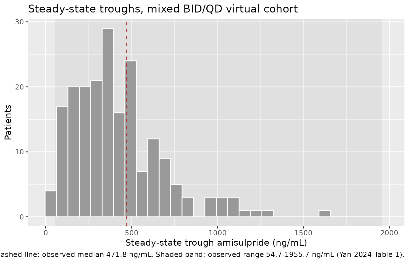

Simulated steady-state trough distribution against the observed median and range of Yan 2024 Table 1.

Renal-function dependence of clearance

cl_by_subj <- sim |> distinct(id, CRCL, cl)
stopifnot(nrow(cl_by_subj) == n_subj)

ggplot(cl_by_subj, aes(CRCL, cl)) +
  geom_point(alpha = 0.4) +
  stat_function(fun = function(x) 45.1 * (x / 114.42)^0.364,
                colour = "firebrick", linewidth = 1) +
  labs(x = "eCLcr (mL/min)", y = "Individual CL/F (L/h)",
       title = "Apparent clearance vs estimated creatinine clearance",
       caption = "Red line: typical-value relationship from Yan 2024 Table 5; points scatter around it by the IIV (omega = 0.207).")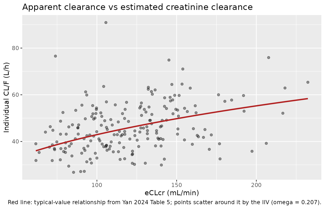

Reproduces the Yan 2024 Table 5 covariate relationship CL/F = 45.1 * (eCLcr/114.42)^0.364.

# The typical-value curve must pass through 45.1 L/h at the centring value and
# reproduce the published exponent over the observed eCLcr range.
mod_typ <- rxode2::zeroRe(mod)
#> ℹ parameter labels from comments will be replaced by 'label()'
typ_ev  <- tibble(
  id   = 1:3,
  CRCL = c(23.29, 114.42, 239.51)
) |>
  tidyr::crossing(tibble(time = c(0, 12), amt = c(300, NA_real_),
                         evid = c(1L, 0L), cmt = c("depot", "central")))

typ <- rxode2::rxSolve(mod_typ, events = typ_ev, keep = "CRCL",
                       useLinCmt = FALSE) |>
  as.data.frame() |>
  distinct(id, CRCL, cl)
#> ℹ omega/sigma items treated as zero: 'etalcl'
#> Warning: multi-subject simulation without without 'omega'

typ |>
  mutate(`Published CL/F (L/h)` = 45.1 * (CRCL / 114.42)^0.364,
         `Model CL/F (L/h)`     = cl) |>
  transmute(`eCLcr (mL/min)` = round(CRCL, 2),
            `Published CL/F (L/h)` = round(`Published CL/F (L/h)`, 3),
            `Model CL/F (L/h)`     = round(`Model CL/F (L/h)`, 3)) |>
  knitr::kable(caption = "Typical-value clearance at the extremes and centre of the observed eCLcr range.")

Typical-value clearance at the extremes and centre of the observed eCLcr range.

eCLcr (mL/min)	Published CL/F (L/h)	Model CL/F (L/h)
23.29	25.266	25.266
114.42	45.100	45.100
239.51	59.014	59.014

stopifnot(max(abs(typ$cl - 45.1 * (typ$CRCL / 114.42)^0.364)) < 1e-6)

Residual-scale check

The Phase-4 reading of Table 5 (IIV = variance, residual = SD) is re-tested here end-to-end: the three competing readings are pushed through the full model and their steady-state trough spreads compared against the observed one. Only the adopted reading reproduces the observed dispersion.

spread_under <- function(omega_var, prop_sd, seed = 11L) {
  m <- readModelDb("Yan_2024_amisulpride")
  m <- eval(bquote(rxode2::ini(m, propSd = .(prop_sd))))
  m <- eval(bquote(rxode2::ini(m, etalcl ~ .(omega_var))))
  set.seed(seed)
  s <- rxode2::rxSolve(m, events = events, keep = "dose_mg_day",
                       useLinCmt = FALSE) |>
    as.data.frame()
  stopifnot(nrow(s) == n_subj)
  dc <- s$sim / s$dose_mg_day
  100 * sd(dc) / mean(dc)
}

scale_check <- tibble::tibble(
  Reading = c(
    "Adopted: IIV = variance 0.043, residual = SD 0.314",
    "Both variances: IIV = 0.043, residual SD = sqrt(0.314) = 0.560",
    "Both SDs: IIV variance = 0.043^2 = 0.0018, residual = SD 0.314"
  ),
  `Simulated CV (%)` = c(
    spread_under(0.043,   0.314),
    spread_under(0.043,   sqrt(0.314)),
    spread_under(0.043^2, 0.314)
  )
) |>
  mutate(
    `Observed CV (%)` = 48.9,
    `Absolute error`  = round(abs(`Simulated CV (%)` - 48.9), 1),
    `Simulated CV (%)` = round(`Simulated CV (%)`, 1)
  )
#> ℹ parameter labels from comments will be replaced by 'label()'
#> ℹ change initial estimate of `propSd` to `0.314`
#> ℹ change initial estimate of `etalcl` to `0.043`
#> ℹ parameter labels from comments will be replaced by 'label()'
#> ℹ change initial estimate of `propSd` to `0.560357029044876`
#> ℹ change initial estimate of `etalcl` to `0.043`
#> ℹ parameter labels from comments will be replaced by 'label()'
#> ℹ change initial estimate of `propSd` to `0.314`
#> ℹ change initial estimate of `etalcl` to `0.001849`

knitr::kable(
  scale_check,
  caption = "Dose-corrected steady-state trough CV under each reading of Yan 2024 Table 5, against the observed 48.9% (Table 1: mean 0.970 +/- 0.474 ng/mL per mg/day)."
)

Dose-corrected steady-state trough CV under each reading of Yan 2024 Table 5, against the observed 48.9% (Table 1: mean 0.970 +/- 0.474 ng/mL per mg/day).

Reading	Simulated CV (%)	Observed CV (%)	Absolute error
Adopted: IIV = variance 0.043, residual = SD 0.314	40.6	48.9	8.3
Both variances: IIV = 0.043, residual SD = sqrt(0.314) = 0.560	60.9	48.9	12.0
Both SDs: IIV variance = 0.043^2 = 0.0018, residual = SD 0.314	36.4	48.9	12.5

# The adopted reading must be the closest of the three to the observed spread,
# and must not exceed the observed total (an unexplained-variability term
# cannot be wider than the data it failed to explain).
stopifnot(which.min(scale_check$`Absolute error`) == 1L)
stopifnot(scale_check$`Simulated CV (%)`[1] < 48.9)
stopifnot(scale_check$`Simulated CV (%)`[2] > 48.9)

The observed dose-corrected CV still contains the QD/BID regimen split and the eCLcr spread, both of which the model explains, so the simulated CV should land slightly below 48.9%. The adopted reading does. The “both variances” reading overshoots the total observed variability, which is impossible for an unexplained-variability term; the “both SDs” reading is far too tight.

PKNCA validation

The paper reports no NCA parameters, so PKNCA is used here to check the model’s internal consistency at steady state: AUC(0-tau) must equal dose / (CL/F) per subject, and Cav must equal AUC(0-tau)/tau.

nca_subj <- subj |> slice_head(n = 120L)

nca_events <- bind_rows(lapply(split(nca_subj, nca_subj$regimen), function(df) {
  tau_i    <- df$tau[[1]]
  dt       <- seq(0, 10 * 24 - tau_i, by = tau_i)
  ot       <- seq(10 * 24 - tau_i, 10 * 24, length.out = 97)
  keys     <- df |> select(id, regimen, dose_mg_day, CRCL, tau, amt_per_dose)
  bind_rows(
    tidyr::crossing(keys, time = dt) |>
      transmute(id, regimen, dose_mg_day, CRCL, tau, time,
                amt = amt_per_dose, evid = 1L, cmt = "depot"),
    tidyr::crossing(keys, time = ot) |>
      transmute(id, regimen, dose_mg_day, CRCL, tau, time,
                amt = NA_real_, evid = 0L, cmt = "central")
  )
})) |>
  arrange(id, time, desc(evid))

nca_sim <- rxode2::rxSolve(mod, events = nca_events,
                           keep = c("regimen", "dose_mg_day", "tau"),
                           useLinCmt = FALSE) |>
  as.data.frame()
stopifnot(length(unique(nca_sim$id)) == nrow(nca_subj))

# Shift each subject onto a common 0-tau window so PKNCA integrates the
# steady-state dosing interval. The filter is `!is.na(Cc)` only - adding
# `time > 0` or `Cc > 0` would drop the interval-start record PKNCA needs.
sim_nca <- nca_sim |>
  filter(!is.na(Cc)) |>
  group_by(id) |>
  mutate(time = time - min(time)) |>
  ungroup() |>
  select(id, time, Cc, regimen)

dose_nca <- nca_subj |>
  transmute(id, time = 0, amt = amt_per_dose, regimen)

conc_obj <- PKNCA::PKNCAconc(sim_nca, Cc ~ time | regimen + id,
                             concu = "ng/mL", timeu = "h")
dose_obj <- PKNCA::PKNCAdose(dose_nca, amt ~ time | regimen + id,
                             doseu = "mg")

# One interval per regimen, each spanning that regimen's own tau.
intervals <- data.frame(
  regimen = c("BID", "QD"),
  start   = 0,
  end     = c(12, 24),
  cmax    = TRUE,
  tmax    = TRUE,
  cmin    = TRUE,
  auclast = TRUE,
  cav     = TRUE
)

nca_res <- PKNCA::pk.nca(PKNCA::PKNCAdata(conc_obj, dose_obj, intervals = intervals))

nca_wide <- as.data.frame(nca_res$result) |>
  filter(PPTESTCD %in% c("auclast", "cav", "cmax", "cmin", "tmax")) |>
  select(id, regimen, PPTESTCD, PPORRES) |>
  pivot_wider(names_from = PPTESTCD, values_from = PPORRES)

check <- nca_wide |>
  inner_join(nca_subj |> select(id, amt_per_dose, tau), by = "id") |>
  inner_join(nca_sim |> distinct(id, cl), by = "id") |>
  mutate(
    # dose (mg) / CL (L/h) = mg*h/L = ug*h/mL; x1000 -> ng*h/mL
    auc_expected = amt_per_dose / cl * 1000,
    auc_pct_err  = 100 * (auclast - auc_expected) / auc_expected,
    cav_pct_err  = 100 * (cav - auclast / tau) / (auclast / tau)
  )
stopifnot(nrow(check) == nrow(nca_subj))

tibble::tibble(
  Check = c("AUC(0-tau) vs dose/(CL/F), per subject",
            "Cav vs AUC(0-tau)/tau, per subject"),
  `Median % error` = c(median(check$auc_pct_err), median(check$cav_pct_err)),
  `Max abs(% error)` = c(max(abs(check$auc_pct_err)), max(abs(check$cav_pct_err)))
) |>
  mutate(across(where(is.numeric), \(x) round(x, 4))) |>
  knitr::kable(caption = "Steady-state mass-balance identities, per subject. AUC(0-tau) is trapezoidal over a 97-point grid, so a small negative bias against the exact dose/CL is expected.")

Steady-state mass-balance identities, per subject. AUC(0-tau) is trapezoidal over a 97-point grid, so a small negative bias against the exact dose/CL is expected.

Check	Median % error	Max abs(% error)
AUC(0-tau) vs dose/(CL/F), per subject	-0.0026	0.0166
Cav vs AUC(0-tau)/tau, per subject	0.0000	0.0000

# Tolerances are set to the accuracy actually achieved on a 97-point grid, so a
# future regression in the ODE or in the unit scaling goes red rather than green.
stopifnot(max(abs(check$auc_pct_err)) < 0.1)
stopifnot(max(abs(check$cav_pct_err)) < 1e-6)

nca_wide |>
  group_by(regimen) |>
  summarise(
    n                    = dplyr::n(),
    `Cmax (ng/mL)`       = median(cmax),
    `Cmin (ng/mL)`       = median(cmin),
    `Cav (ng/mL)`        = median(cav),
    `AUC0-tau (ng*h/mL)` = median(auclast),
    `Peak:trough ratio`  = median(cmax / cmin),
    .groups              = "drop"
  ) |>
  mutate(across(where(is.numeric), \(x) signif(x, 3))) |>
  dplyr::rename("Regimen" = regimen, "N" = n) |>
  knitr::kable(caption = "Median steady-state exposure by regimen in the virtual cohort.")

Median steady-state exposure by regimen in the virtual cohort.

Regimen	N	Cmax (ng/mL)	Cmin (ng/mL)	Cav (ng/mL)	AUC0-tau (ng*h/mL)	Peak:trough ratio
BID	102	572	416	515	6180	1.36
QD	18	784	256	548	13100	3.05

For the same daily dose the once-daily arm has a lower trough and a much larger peak-to-trough swing, which is the pharmacokinetic reason the source cohort is predominantly twice daily.

Remedial strategies for a delayed dose

Yan 2024’s clinical output is a set of remedial regimens for a delayed or missed dose, scored by the percentage of time within the therapeutic range, defined as the interval from the 5th-percentile steady-state trough to the 95th-percentile steady-state peak of the same regimen (Methods, “Nonadherence Scenarios and Remedial Strategies”). The six strategies are reproduced below for the cohort-median regimen of 300 mg twice daily, together with a “no remedial action” reference.

rem_n   <- 100L
rem_amt <- 300   # mg per dose = the cohort-median 600 mg/day given BID
rem_tau <- 12
t_miss  <- 7 * 24   # the dose scheduled for t = 168 h is the one that is delayed
horizon <- 48       # h of follow-up scored after that scheduled time

set.seed(4242)
rem_subj <- tibble(id = seq_len(rem_n), CRCL = draw_crcl(rem_n))

# frac_now  = fraction of a regular dose taken when the patient remembers
# frac_next = fraction taken at the next scheduled time
# skip_next = drop the next scheduled dose entirely
strategies <- tibble::tribble(
  ~strategy, ~label,                                              ~frac_now, ~frac_next, ~skip_next,
  "none",    "None: skip the dose, resume the schedule",               0.0,      1.0,       FALSE,
  "A",       "A: full dose now, full dose at next scheduled",           1.0,      1.0,       FALSE,
  "B",       "B: half dose now, full dose at next scheduled",           0.5,      1.0,       FALSE,
  "C",       "C: full dose now, half dose at next scheduled",           1.0,      0.5,       FALSE,
  "D",       "D: 1.5x dose now, skip next scheduled",                   1.5,      0.0,       TRUE,
  "E",       "E: 1.5x dose now, then resume",                           1.5,      1.0,       FALSE,
  "F",       "F: 2x dose now, then resume",                             2.0,      1.0,       FALSE
)

# Delays are kept strictly inside the 12 h dosing interval: at exactly 12 h the
# remedial dose and the next scheduled dose coincide and several strategies
# collapse onto one another.
delays <- c(3, 6, 11)

make_arm <- function(delay_h, frac_now, frac_next, skip_next, id_offset) {
  s <- rem_subj |> mutate(id = id + id_offset)

  pre  <- seq(0, t_miss - rem_tau, by = rem_tau)          # routine, before the miss
  post <- seq(t_miss + 2 * rem_tau, t_miss + horizon, by = rem_tau)  # routine, after

  rem_times <- c(t_miss + delay_h, t_miss + rem_tau)
  rem_fracs <- c(frac_now, if (skip_next) 0 else frac_next)
  keep      <- rem_fracs > 0

  sched <- tibble(
    time = c(pre, rem_times[keep], post),
    frac = c(rep(1, length(pre)), rem_fracs[keep], rep(1, length(post)))
  ) |>
    group_by(time) |>                       # coincident doses add, they do not duplicate
    summarise(frac = sum(frac), .groups = "drop")

  bind_rows(
    tidyr::crossing(s, sched) |>
      transmute(id, CRCL, time, amt = rem_amt * frac, evid = 1L, cmt = "depot"),
    tidyr::crossing(s, tibble(time = seq(t_miss, t_miss + horizon, by = 0.25))) |>
      transmute(id, CRCL, time, amt = NA_real_, evid = 0L, cmt = "central")
  ) |>
    arrange(id, time, desc(evid))
}

grid <- tidyr::crossing(strategies, delay_h = delays) |>
  mutate(id_offset = (row_number() - 1L) * rem_n)

rem_events <- bind_rows(Map(
  function(d, fn, fx, sk, off, st, lab) {
    make_arm(d, fn, fx, sk, off) |>
      mutate(strategy = st, label = lab, delay_h = d)
  },
  grid$delay_h, grid$frac_now, grid$frac_next, grid$skip_next,
  grid$id_offset, grid$strategy, grid$label
))
stopifnot(!anyDuplicated(unique(rem_events[, c("id", "time", "evid")])))

# Reference arm: the undisturbed BID regimen. Its 5th-percentile trough and
# 95th-percentile peak over the same window define the therapeutic range.
ref_events <- bind_rows(
  tidyr::crossing(rem_subj,
                  tibble(time = seq(0, t_miss + horizon - rem_tau, by = rem_tau))) |>
    transmute(id, CRCL, time, amt = rem_amt, evid = 1L, cmt = "depot"),
  tidyr::crossing(rem_subj,
                  tibble(time = seq(t_miss, t_miss + horizon, by = 0.25))) |>
    transmute(id, CRCL, time, amt = NA_real_, evid = 0L, cmt = "central")
) |>
  arrange(id, time, desc(evid))

ref_sim <- rxode2::rxSolve(mod, events = ref_events, useLinCmt = FALSE) |>
  as.data.frame()

ss <- ref_sim |>
  mutate(interval = floor((time - t_miss) / rem_tau)) |>
  filter(interval >= 0, interval < horizon / rem_tau) |>
  group_by(id, interval) |>
  summarise(peak = max(Cc), trough = min(Cc), .groups = "drop")

tr_low  <- unname(quantile(ss$trough, 0.05))
tr_high <- unname(quantile(ss$peak,   0.95))
round(c(`therapeutic range low (ng/mL)` = tr_low,
        `therapeutic range high (ng/mL)` = tr_high), 1)
#>  therapeutic range low (ng/mL) therapeutic range high (ng/mL) 
#>                          274.2                          848.9

rem_sim <- rxode2::rxSolve(
  mod, events = rem_events,
  keep      = c("strategy", "label", "delay_h"),
  useLinCmt = FALSE
) |>
  as.data.frame()

stopifnot(length(unique(rem_sim$id)) == nrow(grid) * rem_n)

scored <- rem_sim |>
  group_by(strategy, label, delay_h) |>
  summarise(
    `% time in range`    = 100 * mean(Cc >= tr_low & Cc <= tr_high),
    `% time below range` = 100 * mean(Cc < tr_low),
    `% time above range` = 100 * mean(Cc > tr_high),
    .groups = "drop"
  )

fluctuation <- rem_sim |>
  group_by(strategy, label, delay_h, id) |>
  summarise(swing = max(Cc) / min(Cc), .groups = "drop") |>
  group_by(strategy, label, delay_h) |>
  summarise(`Median peak:trough swing` = median(swing),
            `Median Cmax (ng/mL)` = NA_real_, .groups = "drop")

peak_by_arm <- rem_sim |>
  group_by(strategy, delay_h, id) |>
  summarise(cmax = max(Cc), .groups = "drop") |>
  group_by(strategy, delay_h) |>
  summarise(`Median Cmax (ng/mL)` = median(cmax), .groups = "drop")

fluctuation <- fluctuation |>
  select(-`Median Cmax (ng/mL)`) |>
  inner_join(peak_by_arm, by = c("strategy", "delay_h"))

ref_pct <- 100 * mean(ref_sim$Cc >= tr_low & ref_sim$Cc <= tr_high)

scored |>
  mutate(`% time in range` = round(`% time in range`, 1)) |>
  select(label, delay_h, `% time in range`) |>
  pivot_wider(names_from = delay_h, values_from = `% time in range`,
              names_prefix = "Delay ") |>
  dplyr::rename("Strategy" = label) |>
  knitr::kable(caption = sprintf(
    "Percentage of the 48 h following the scheduled dose spent within the therapeutic range (%.0f-%.0f ng/mL). An undisturbed regimen scores %.1f%%.",
    tr_low, tr_high, ref_pct))

Percentage of the 48 h following the scheduled dose spent within the therapeutic range (274-849 ng/mL). An undisturbed regimen scores 96.7%.

Strategy	Delay 3	Delay 6	Delay 11
A: full dose now, full dose at next scheduled	94.7	87.6	82.9
B: half dose now, full dose at next scheduled	93.6	91.7	86.0
C: full dose now, half dose at next scheduled	95.8	94.7	86.3
D: 1.5x dose now, skip next scheduled	93.3	90.9	88.1
E: 1.5x dose now, then resume	87.1	81.2	69.4
F: 2x dose now, then resume	74.0	70.9	57.5
None: skip the dose, resume the schedule	84.3	82.4	84.4

fluctuation |>
  select(label, delay_h, `Median peak:trough swing`, `Median Cmax (ng/mL)`) |>
  mutate(`Median peak:trough swing` = round(`Median peak:trough swing`, 2),
         `Median Cmax (ng/mL)` = round(`Median Cmax (ng/mL)`)) |>
  arrange(delay_h, label) |>
  dplyr::rename("Strategy" = label, "Delay (h)" = delay_h) |>
  knitr::kable(caption = "Fluctuation and peak exposure over the 48 h window, by strategy and delay.")

Fluctuation and peak exposure over the 48 h window, by strategy and delay.

Strategy	Delay (h)	Median peak:trough swing	Median Cmax (ng/mL)
A: full dose now, full dose at next scheduled	3	1.77	658
B: half dose now, full dose at next scheduled	3	1.81	604
C: full dose now, half dose at next scheduled	3	1.67	576
D: 1.5x dose now, skip next scheduled	3	2.42	689
E: 1.5x dose now, then resume	3	2.14	779
F: 2x dose now, then resume	3	2.53	899
None: skip the dose, resume the schedule	3	3.25	589
A: full dose now, full dose at next scheduled	6	2.36	696
B: half dose now, full dose at next scheduled	6	2.10	596
C: full dose now, half dose at next scheduled	6	2.00	597
D: 1.5x dose now, skip next scheduled	6	2.21	627
E: 1.5x dose now, then resume	6	2.93	826
F: 2x dose now, then resume	6	3.36	993
None: skip the dose, resume the schedule	6	3.48	563
A: full dose now, full dose at next scheduled	11	3.87	715
B: half dose now, full dose at next scheduled	11	3.28	625
C: full dose now, half dose at next scheduled	11	3.03	649
D: 1.5x dose now, skip next scheduled	11	3.30	597
E: 1.5x dose now, then resume	11	4.36	896
F: 2x dose now, then resume	11	5.76	1004
None: skip the dose, resume the schedule	11	3.30	583

rem_sim |>
  group_by(label, delay_h, time) |>
  summarise(Q50 = median(Cc), .groups = "drop") |>
  mutate(delay_lab = paste0("Delay ", delay_h, " h")) |>
  ggplot(aes(time - t_miss, Q50, colour = label)) +
  annotate("rect", xmin = -Inf, xmax = Inf, ymin = tr_low, ymax = tr_high, alpha = 0.12) +
  geom_line() +
  facet_wrap(~delay_lab, ncol = 1) +
  labs(x = "Time after the scheduled (missed) dose (h)",
       y = "Median amisulpride (ng/mL)", colour = NULL,
       title = "Remedial strategies after a delayed 300 mg BID dose",
       caption = "Reproduces the design of Yan 2024 Supplementary Figure S5.") +
  theme(legend.position = "bottom", legend.text = element_text(size = 7)) +
  guides(colour = guide_legend(ncol = 2))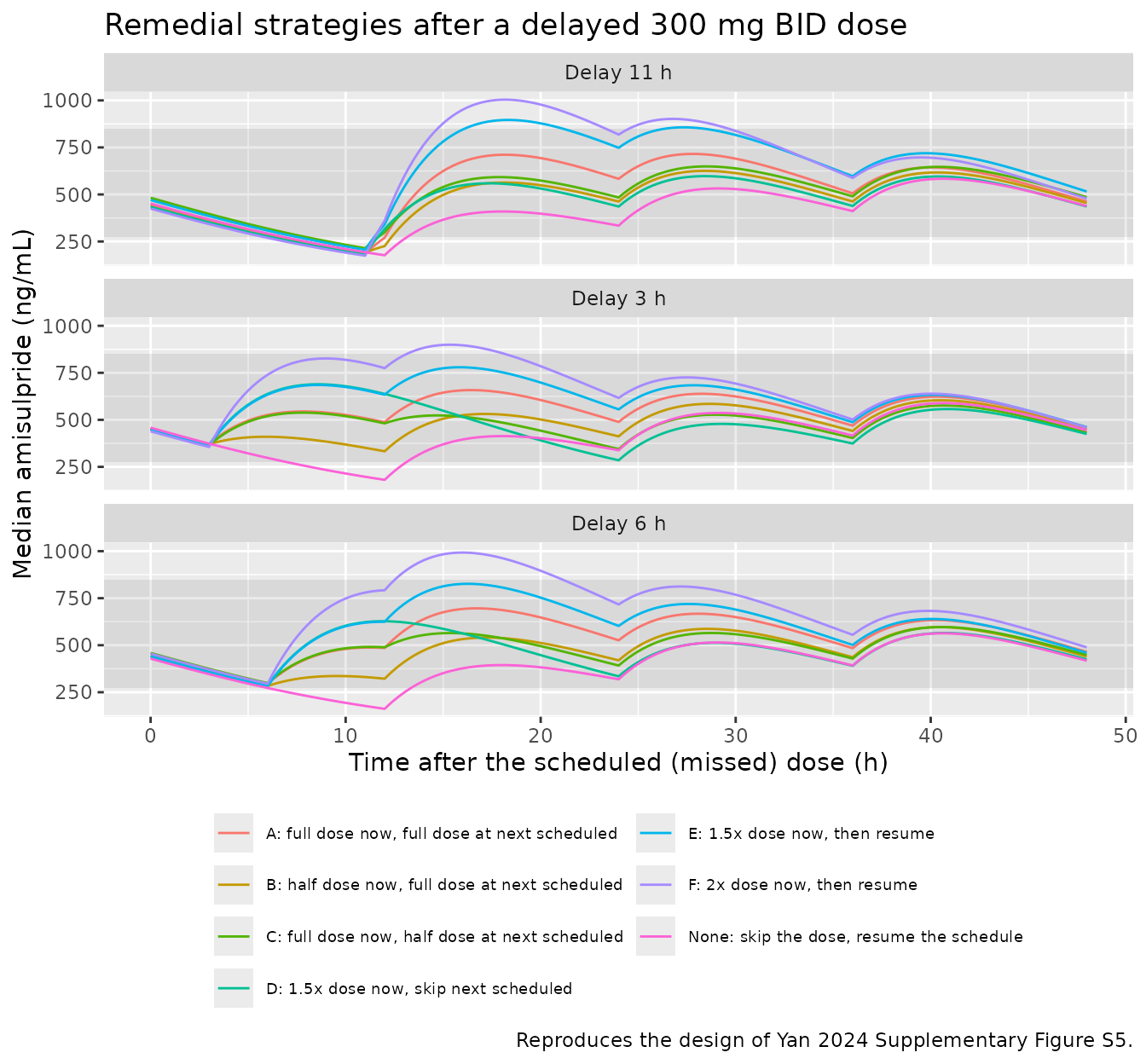

Median concentration-time profiles after a delayed dose under each remedial strategy. Shaded band: the therapeutic range.

Four of the paper’s qualitative claims survive as testable statements about the packaged model. Each is checked at every simulated delay.

by_delay <- function(f) all(vapply(delays, f, logical(1)))

worst_in_range <- function(d) {
  s <- scored[scored$delay_h == d, ]
  s$strategy[which.min(s$`% time in range`)]
}
none_score <- function(d) scored$`% time in range`[scored$delay_h == d & scored$strategy == "none"]

claims <- tibble::tibble(
  Claim = c(
    "Taking no remedial action is never the best option (Results: a remedial regimen is always advised)",
    "B, C and D - the strategies that replace exactly half a dose - all beat taking no action",
    "Front-loading a double dose (F) is the worst strategy on time in range (Discussion: 'excessively high blood concentrations')",
    "Among the six remedial strategies, F gives both the highest peak and the largest fluctuation"
  ),
  Holds = c(
    by_delay(function(d) worst_in_range(d) != "none" &&
               max(scored$`% time in range`[scored$delay_h == d]) > none_score(d)),
    by_delay(function(d) {
      s <- scored[scored$delay_h == d, ]
      all(s$`% time in range`[s$strategy %in% c("B", "C", "D")] > none_score(d))
    }),
    by_delay(function(d) worst_in_range(d) == "F"),
    by_delay(function(d) {
      # "none" is the do-nothing baseline, not a remedial strategy; it is
      # excluded here because skipping the dose outright produces the deepest
      # trough and therefore a large swing of its own (see the table above).
      f <- fluctuation[fluctuation$delay_h == d & fluctuation$strategy != "none", ]
      f$strategy[which.max(f$`Median Cmax (ng/mL)`)] == "F" &&
        f$strategy[which.max(f$`Median peak:trough swing`)] == "F"
    })
  )
)
knitr::kable(claims, caption = "Yan 2024 qualitative claims about the remedial strategies, tested against the packaged model.")

Yan 2024 qualitative claims about the remedial strategies, tested against the packaged model.

Claim	Holds
Taking no remedial action is never the best option (Results: a remedial regimen is always advised)	TRUE
B, C and D - the strategies that replace exactly half a dose - all beat taking no action	TRUE
Front-loading a double dose (F) is the worst strategy on time in range (Discussion: ‘excessively high blood concentrations’)	TRUE
Among the six remedial strategies, F gives both the highest peak and the largest fluctuation	TRUE

stopifnot(all(claims$Holds))

best <- scored |>
  filter(strategy != "none") |>
  group_by(delay_h) |>
  slice_max(`% time in range`, n = 2, with_ties = FALSE) |>
  mutate(rank = row_number()) |>
  ungroup() |>
  transmute(`Delay (h)` = delay_h, Rank = rank, Strategy = label,
            `% time in range` = round(`% time in range`, 1))
knitr::kable(best, caption = "Two highest-scoring remedial strategies by delay, under the time-in-range metric as implemented here.")

Two highest-scoring remedial strategies by delay, under the time-in-range metric as implemented here.

Delay (h)	Rank	Strategy	% time in range
3	1	C: full dose now, half dose at next scheduled	95.8
3	2	A: full dose now, full dose at next scheduled	94.7
6	1	C: full dose now, half dose at next scheduled	94.7
6	2	B: half dose now, full dose at next scheduled	91.7
11	1	D: 1.5x dose now, skip next scheduled	88.1
11	2	C: full dose now, half dose at next scheduled	86.3

The ranking should be read alongside, not as a substitute for, the paper’s recommendation. Yan 2024 recommends Strategy B (half the missed dose immediately, then resume) for a delay of up to 12 h, and names B and C as the two candidates for the 6-12 h window - which is what the metric returns at the 6 h delay here. It does not return B at the shortest delay, and that is expected: a pure time-in-range score rewards replacing the missing exposure as completely as possible, whereas the paper’s preference for the more conservative option is argued on safety grounds that this metric does not encode - amisulpride’s concentration-dependent QTc prolongation, which is driven by the peak rather than by time in range. Those peak consequences are exactly what the fluctuation table and the figure show, and they are the reason the double-dose strategy F is both the highest-peaking and the lowest-scoring arm at every delay.

The fluctuation table also makes the cost of not acting explicit: at the 3 h and 6 h delays the do-nothing baseline swings more than any remedial strategy except F, because the skipped dose leaves an unusually deep trough before the next scheduled dose arrives.

Assumptions and deviations

• eCLcr centring value (114.42 mL/min) is not printed in Table 5. It is recovered from the Discussion sentence “the typical clearance rate of amisulpride is 45.1 L/h (average eCLcr 114.42 mL/min)” read together with the Table 1 eCLcr row, whose median is exactly 114.42. The same power-on-cohort-median form is used by the two amisulpride models this one was built from (Table 3, models M1 and M5).
• Table 5 mixes variance and SD conventions. The IIV row (0.043) is a variance and the residual row (0.314) is a standard deviation; neither is labelled. Both scales were established from the paper’s own Figure 1 rather than assumed - see How the two variability scales were resolved for the digitisation and the residual-scale check for the end-to-end confirmation. The Methods sentence describing the residual as having “sigma variance” is inconsistent with the model actually fitted, as Figure 1E shows, and was not followed.
• The five externally evaluated models (M1-M5) are not extracted from this paper. Yan 2024 Table 3 transcribes them, but that transcription is demonstrably unreliable: model M4’s clearance is printed as 1.04 * (AGE/32)^-0.624 L/h, which contradicts the paper’s own Results text that “typical estimates for amisulpride clearance in the included studies ranged from 32.6 to 61.1 L/h”; the IIV column lists three to five bare percentages per model with no indication of which parameter each belongs to; and the study labels in Tables 2 and 3 give the authors’ given names rather than their surnames (M1 “Wei L.” is Liu W, M3 “Anais G.” is Glatard A, and so on). Extracting from a secondary summary table would also discard each primary paper’s covariate encodings, reference categories and residual structure. The primary papers should be extracted individually: Liu 2023 (doi:10.5414/CP204334), Reeves 2016 (doi:10.1007/s00213-016-4379-6), Glatard 2020 (doi:10.1007/s40262-019-00821-w), Huang 2021 (doi:10.2147/DDDT.S327506) and Li 2023 (doi:10.3389/fphar.2023.1215065).
• The virtual cohort’s dose distribution is assumed. Table 1 gives only the median (600 mg/day), mean (555.90 +/- 192.56) and range of daily dose, not the per-patient histogram. A six-level discrete distribution reproducing the published median and mean is used; its SD (about 220 mg/day) is somewhat wider than the published 192.56.
• The Results text and Table 1 disagree on the dose range. The Results narrative states “a daily dosage range of 200-2000 mg (median = 600 mg)” while Table 1 prints 600(200,1200). The Table 1 range is used, here and in the model’s population metadata.
• The sample-to-dose gap is not published and is assumed. Yan 2024 states only that blood was drawn at 06:00 “prior to the next dose”; it gives neither the per-patient dosing clock times nor the measured gap between the last dose and the sample. Simulating an exact end-of-interval trough under-predicts the observed concentration statistic by about a quarter, and a 2 h gap (a conventional 08:00 / 20:00 twice-daily schedule sampled at 06:00) recovers roughly half of that. The model’s average steady-state exposure, which does not depend on this assumption, matches the observed concentrations to within a few percent; see the Cavg check.
• eCLcr is treated as time-fixed per subject, matching the source analysis (390 observations from 361 patients, so nearly one TDM occasion each).
• The therapeutic range is computed at the cohort level. Yan 2024 defines it as “the concentration interval spanning from the 5th percentile trough concentration to the 95th percentile peak concentration at the steady state of a given dose” and calls it an individual therapeutic range; the percentiles here are taken across the virtual cohort at the cohort-median 300 mg BID regimen. The 48 h scoring window is a choice - the paper does not state one.
• Delays are simulated at 3, 6 and 11 h. These bracket the paper’s 6 h and 12 h decision points while staying strictly inside the 12 h dosing interval; at exactly 12 h the remedial dose coincides with the next scheduled dose and several strategies become identical. The paper’s “delay beyond 24 h” recommendation - skip the missed dose and resume the routine schedule - is the “None” row of the tables above.
• No IIV on V/F and no additive residual term are encoded, because Table 5 reports neither. With trough-only data V/F is weakly identified (RSE 20%, bootstrap 95% CI 319.5-742.0 L).
• Bioavailability is not separately identifiable. All disposition parameters are apparent (CL/F, V/F) and the nominal dose enters the depot compartment unscaled. Amisulpride’s absolute bioavailability of about 48% (Introduction) is not part of this model.
• The supplementary material (Figures S1-S5, Tables S1-S2) was not available on disk. It holds the covariate-screening steps and the diagnostic panels for the five evaluated models; none of it contributes parameter values to the packaged model, all of which come from Table 5 and the main-text Discussion.