Cyclosporin (Wang 2019)
Source:vignettes/articles/Wang_2019_cyclosporin.Rmd
Wang_2019_cyclosporin.RmdModel and source
- Citation: Wang DD, Chen X, Li ZP. Cyclosporin population pharmacokinetics in pediatric refractory nephrotic syndrome based on real-world studies: Effects of body weight and spirolactone administration. Exp Ther Med. 2019;17(4):3015-3020. doi:10.3892/etm.2019.7325
- Description: One-compartment first-order-absorption population PK model for oral cyclosporin in Chinese children with pediatric refractory nephrotic syndrome, with allometric body weight on CL/F and V/F and a concomitant-spironolactone effect on CL/F (Wang 2019)
- Article: https://doi.org/10.3892/etm.2019.7325
Wang, Chen and Li (2019) built the first population PK model for
cyclosporin in pediatric refractory nephrotic syndrome (PRNS), using a
retrospective real-world therapeutic-drug-monitoring (TDM) dataset of 18
Chinese children treated at the Children’s Hospital of Fudan University
between June 2014 and June 2018. Every modelled concentration was a
whole-blood trough, so neither bioavailability nor an absorption lag was
estimable and the absorption rate constant was fixed at 0.68 1/h from
the Ni 2013 pediatric ciclosporin model (Wang 2019 reference 9, already
in this library as Ni_2013_ciclosporin). The structural
model is a one-compartment model with first-order absorption and
first-order elimination, parameterised in apparent (F-scaled) terms CL/F
and V/F.
The final covariate model (Wang 2019 Results) is
i.e. allometric body weight on both disposition parameters at a 70 kg
adult reference, plus a 26.5% reduction in apparent oral clearance when
spironolactone is coadministered. The paper spells the interacting drug
“spirolactone” throughout; the rINN is spironolactone, and the model
file uses the canonical covariate column CONMED_SPIRON.
Population
Wang 2019 Table I summarises the cohort: n = 18 children (13 male / 5 female; 27.8% female), age 2.79 +/- 0.90 years (median 2.75, range 1.18-4.57), body weight 15.28 +/- 2.95 kg (median 15, range 10-23), height 91.28 +/- 8.23 cm (median 94, range 77-105). The cohort is markedly hypoalbuminaemic (albumin 19.68 +/- 6.82 g/L), as expected in nephrotic syndrome, with preserved renal function (creatinine median 20.5 umol/L; patients with diagnosed kidney failure were excluded per Fig. 1). Cyclosporin was given orally as a liquid solution at an initial 25-80 mg daily, subsequently adjusted on clinical response, adverse events and TDM trough concentration.
Wang 2019 Table II gives the concomitant-medication counts: spironolactone 11/18, prednisolone 13/18, piperazine ferulate 5/18, methylprednisolone 4/18, diltiazem 3/18, fosinopril 3/18, dipyridamole 2/18, felodipine 1/18, nifedipine 1/18. Only spironolactone was retained in the final covariate model.
The same information is available programmatically via the model’s
population metadata
(rxode2::rxode(readModelDb("Wang_2019_cyclosporin"))$meta$population).
Source trace
The per-parameter origin is recorded as an in-file comment next to
each ini() entry in
inst/modeldb/specificDrugs/Wang_2019_cyclosporin.R. The
table below collects them in one place for review.
| Equation / parameter | Value | Source location |
|---|---|---|
lka (Ka) |
fixed(log(0.68)) (1/h) |
Wang 2019 Methods ‘PPK modeling’; Table III ‘Ka (h-1) 0.68 (fixed)’ |
lcl (CL/F at WT = 70 kg, no spironolactone) |
log(80.7) (L/h) |
Wang 2019 Table III ‘CL/F (L/h)’; Abstract |
lvc (V/F at WT = 70 kg) |
log(2030) (L) |
Wang 2019 Table III ‘V/F (L)’; Abstract |
e_wt_cl (allometric CL/F exponent) |
fixed(0.75) |
Wang 2019 Methods ‘Covariate model’ (PWR = 0.75 for CL/F; reference 15) |
e_wt_vc (allometric V/F exponent) |
fixed(1.0) |
Wang 2019 Methods ‘Covariate model’ (PWR = 1 for V/F; reference 15) |
e_conmed_spiron_cl (spironolactone) |
-0.265 |
Wang 2019 Table III ‘theta-spirolactone’; Results equation |
| IIV CL/F (omega = 0.446, 44.6%) | etalcl ~ 0.446^2 = 0.198916 |
Wang 2019 Table III ‘omega CL/F’; Abstract quotes it as 44.6% |
| IIV V/F (omega = 0.531, 53.1%) | etalvc ~ 0.531^2 = 0.281961 |
Wang 2019 Table III ‘omega V/F’; Abstract quotes it as 53.1% |
| Residual proportional |
propSd = 0.117 (11.7%) |
Wang 2019 Table III ‘sigma1’ (proportional error) |
| Residual additive |
addSd = 8.062 (ng/mL) |
Wang 2019 Table III ‘sigma2’ (additive error) |
| Allometric reference body weight | 70 kg | Wang 2019 Methods ‘Covariate model’ (WTstd = 70 kg) |
| Structural model | 1-cmt oral, first-order absorption and elimination | Wang 2019 Results ‘Modeling’; Abstract |
| IIV model | exponential, Pi = T(P) * exp(eta_i)
|
Wang 2019 Methods ‘Random-effects model’ |
| Residual model | combined, OB = IP * (1 + eps1) + eps2
|
Wang 2019 Methods ‘Random-effects model’ |
| Concentration unit conversion | Cc <- central / vc * 1000 |
Derived: dose in mg and V/F in L give mg/L; x1000 -> ng/mL, the assay/Table III unit |
Setup
mod <- readModelDb("Wang_2019_cyclosporin")
ui <- rxode2::rxode(mod)
mod_typical <- mod |> rxode2::zeroRe()

# The model declares explicit ODE states. rxode2 will silently replace an
# explicit ODE system with its closed-form linCmt() solution when the
# parameterisation allows it, which would make every check below a test of
# rxode2's analytic solver rather than of the encoded ODEs. Assert the
# states survive.
stopifnot(identical(ui$state, c("depot", "central")))
Structural gate: the encoded covariate equations
The first check is arithmetic, not simulation: evaluate the model’s
derived cl and vc over a grid spanning the
cohort weight range with and without spironolactone, and compare against
the published equations coded independently. This is a deterministic
identity, so it is asserted to solver precision.
grid <- tidyr::expand_grid(
  WT = c(10, 15, 23, 70),
  CONMED_SPIRON = c(0, 1)
) |>
  dplyr::mutate(id = dplyr::row_number())

# Published equations, transcribed independently of the model file.
published_cl <- function(wt, spiron) 80.7 * (wt / 70)^0.75 * (1 + spiron * -0.265)
published_vc <- function(wt, spiron) 2030 * (wt / 70)^1

ev_grid <- dplyr::bind_rows(lapply(seq_len(nrow(grid)), function(i) {
  row <- grid[i, ]
  out <- tibble::tibble(
    id = row$id,
    time = c(0, 1),
    evid = c(1L, 0L),
    amt = c(25, NA_real_),
    cmt = c("depot", "central")
  )
  out$WT <- row$WT
  out$CONMED_SPIRON <- row$CONMED_SPIRON
  out
}))

sim_grid <- rxode2::rxSolve(
  mod_typical,
  events = ev_grid,
  keep = c("WT", "CONMED_SPIRON")
) |>
  as.data.frame() |>
  dplyr::group_by(id) |>
  dplyr::slice_tail(n = 1) |>
  dplyr::ungroup() |>
  dplyr::mutate(
    cl_pub = published_cl(WT, CONMED_SPIRON),
    vc_pub = published_vc(WT, CONMED_SPIRON),
    cl_relerr = abs(cl / cl_pub - 1),
    vc_relerr = abs(vc / vc_pub - 1)
  )
#> ℹ omega/sigma items treated as zero: 'etalcl', 'etalvc'
#> Warning: multi-subject simulation without without 'omega'

# The gate must have rows to test (a zero-row filter makes all() vacuously
# TRUE), and the identity is exact arithmetic, not a cohort statistic.
stopifnot(
  nrow(sim_grid) == nrow(grid),
  all(sim_grid$cl_relerr < 1e-10),
  all(sim_grid$vc_relerr < 1e-10)
)

sim_grid |>
  dplyr::select(WT, CONMED_SPIRON, cl, cl_pub, vc, vc_pub) |>
  dplyr::rename(
    "WT (kg)" = WT,
    "Spironolactone" = CONMED_SPIRON,
    "CL/F model (L/h)" = cl,
    "CL/F published (L/h)" = cl_pub,
    "V/F model (L)" = vc,
    "V/F published (L)" = vc_pub
  ) |>
  knitr::kable(
    digits = 3,
    caption = "Model-derived CL/F and V/F versus the Wang 2019 Results equations across the cohort weight range."
)| WT (kg) | Spironolactone | CL/F model (L/h) | CL/F published (L/h) | V/F model (L) | V/F published (L) |
|---|---|---|---|---|---|
| 10 | 0 | 18.752 | 18.752 | 290 | 290 |
| 10 | 1 | 13.783 | 13.783 | 290 | 290 |
| 15 | 0 | 25.417 | 25.417 | 435 | 435 |
| 15 | 1 | 18.681 | 18.681 | 435 | 435 |
| 23 | 0 | 35.022 | 35.022 | 667 | 667 |
| 23 | 1 | 25.741 | 25.741 | 667 | 667 |
| 70 | 0 | 80.700 | 80.700 | 2030 | 2030 |
| 70 | 1 | 59.314 | 59.315 | 2030 | 2030 |
A gate that cannot go red is worse than none, so confirm the comparison actually discriminates: perturbing the published volume by 1% must break it.
mutation_relerr <- abs(sim_grid$vc / (sim_grid$vc_pub * 1.01) - 1)
stopifnot(all(mutation_relerr > 1e-3))
cat(sprintf(
  "Mutation control: a 1%% error in V/F gives relative deviation %.4f (gate threshold 1e-10).\n",
  max(mutation_relerr)
))
#> Mutation control: a 1% error in V/F gives relative deviation 0.0099 (gate threshold 1e-10).
Closed-form gate: the one-compartment oral solution
For a single oral dose into depot with first-order
absorption and elimination, the typical-value concentration has the
closed form
Both sides use the same parameters, so the discrepancy is pure numerical error and a tight bound is the correct assertion.
wt_ref <- 15 # cohort median body weight, Wang 2019 Table I
dose_mg <- 25 # a single dose of the published 25-80 mg daily range

closed_form <- function(t, dose, wt, spiron) {
  cl <- published_cl(wt, spiron)
  vc <- published_vc(wt, spiron)
  ka <- 0.68
  kel <- cl / vc
  dose / vc * ka / (ka - kel) * (exp(-kel * t) - exp(-ka * t)) * 1000
}

# A log-spaced early grid resolves the absorption phase; a coarse grid
# alone understates Cmax and AUC by several percent.
t_grid <- sort(unique(c(
  0,
  exp(seq(log(0.05), log(4), length.out = 60)),
  seq(4, 96, by = 0.5)
)))

ev_cf <- dplyr::bind_rows(lapply(c(0, 1), function(spiron) {
  out <- tibble::tibble(
    id = spiron + 1L,
    time = c(0, t_grid),
    evid = c(1L, rep(0L, length(t_grid))),
    amt = c(dose_mg, rep(NA_real_, length(t_grid))),
    cmt = c("depot", rep("central", length(t_grid)))
  )
  out$WT <- wt_ref
  out$CONMED_SPIRON <- spiron
  out
}))

sim_cf <- rxode2::rxSolve(
  mod_typical,
  events = ev_cf,
  keep = c("WT", "CONMED_SPIRON")
) |>
  as.data.frame() |>
  dplyr::filter(time > 0) |>
  dplyr::mutate(Cc_closed = closed_form(time, dose_mg, WT, CONMED_SPIRON))
#> ℹ omega/sigma items treated as zero: 'etalcl', 'etalvc'
#> Warning: multi-subject simulation without without 'omega'

# Restrict the relative comparison to concentrations above solver noise;
# the far tail is dominated by absolute tolerance.
cf_check <- sim_cf |>
  dplyr::filter(Cc_closed > 1e-3) |>
  dplyr::mutate(relerr = abs(Cc - Cc_closed) / Cc_closed)

stopifnot(
  nrow(cf_check) > 100,
  all(sim_cf$Cc >= 0),
  max(cf_check$relerr) < 1e-4
)
cat(sprintf(
  "Closed-form gate: %d points compared, max relative error %.2e.\n",
  nrow(cf_check), max(cf_check$relerr)
))
#> Closed-form gate: 488 points compared, max relative error 1.22e-06.
ggplot(
  sim_cf |>
    dplyr::mutate(arm = ifelse(
      CONMED_SPIRON == 1, "with spironolactone", "no spironolactone"
    )),
  aes(time, Cc, colour = arm)
) +
  geom_line(linewidth = 0.9) +
  geom_point(
    data = ~ dplyr::filter(.x, time %in% t_grid[seq(1, length(t_grid), by = 8)]),
    aes(y = Cc_closed), shape = 1, size = 2
  ) +
  labs(
    x = "Time (h)", y = "Whole-blood cyclosporin (ng/mL)", colour = NULL,
    title = "Single 25 mg oral dose, WT = 15 kg"
  ) +
  theme_minimal() +
  theme(legend.position = "top")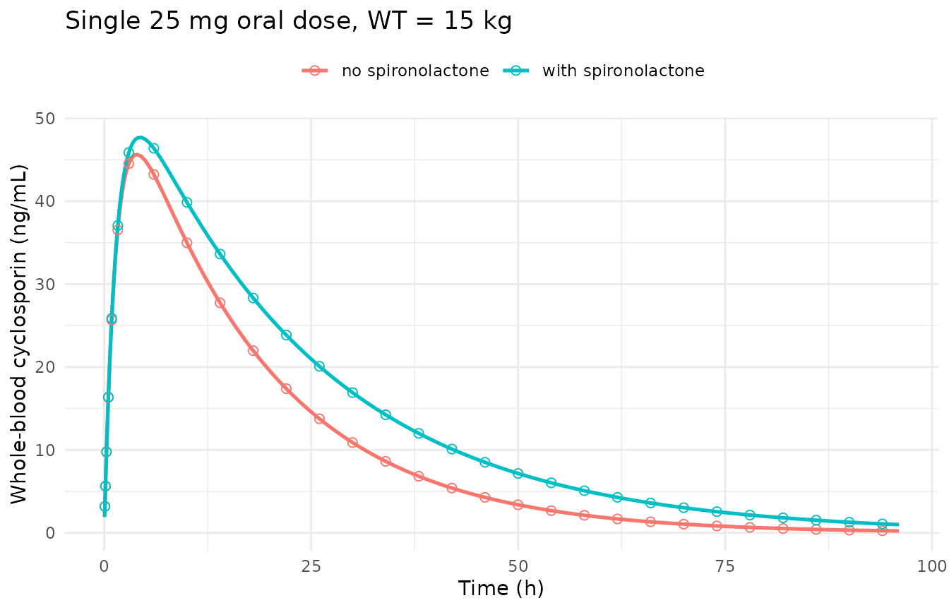
Typical-value single-dose profile for a 15 kg child at 25 mg oral cyclosporin, with and without concomitant spironolactone. Points are the analytic one-compartment oral solution; lines are the rxode2 ODE solve.
Mass-balance gate: dose recovery through CL/F
Because CL/F and V/F are apparent (F-scaled) parameters and the whole
dose enters depot, the identity
CL/F * AUC_inf = Dose must hold exactly for the
typical-value solve. This is computed with PKNCA rather than an inline
trapezoid.
nca_conc <- sim_cf |>
  dplyr::mutate(
    arm = ifelse(CONMED_SPIRON == 1, "with spironolactone", "no spironolactone")
  ) |>
  dplyr::select(id, arm, time, Cc) |>
  dplyr::filter(!is.na(Cc))

# PKNCA needs a record at the start of the interval; the solve grid drops
# time 0 above, so add it back explicitly (C(0) = 0 after an oral dose).
nca_conc <- dplyr::bind_rows(
  nca_conc |>
    dplyr::distinct(id, arm) |>
    dplyr::mutate(time = 0, Cc = 0),
  nca_conc
) |>
  dplyr::arrange(id, time)

conc_obj <- PKNCA::PKNCAconc(
  nca_conc, Cc ~ time | arm + id,
  concu = "ng/mL", timeu = "h"
)

nca_dose <- nca_conc |>
  dplyr::distinct(id, arm) |>
  dplyr::mutate(time = 0, amt = dose_mg)

dose_obj <- PKNCA::PKNCAdose(nca_dose, amt ~ time | arm + id, doseu = "mg")

intervals <- data.frame(
  start = 0, end = Inf,
  cmax = TRUE, tmax = TRUE, half.life = TRUE,
  auclast = TRUE, aucinf.obs = TRUE
)

nca_res <- PKNCA::pk.nca(PKNCA::PKNCAdata(conc_obj, dose_obj, intervals = intervals))
nca_df <- as.data.frame(nca_res$result)

nca_wide <- nca_df |>
  dplyr::select(arm, id, PPTESTCD, PPORRES) |>
  tidyr::pivot_wider(names_from = PPTESTCD, values_from = PPORRES) |>
  dplyr::left_join(
    sim_cf |>
      dplyr::distinct(id, CONMED_SPIRON, WT) |>
      dplyr::mutate(
        cl_pub = published_cl(WT, CONMED_SPIRON),
        vc_pub = published_vc(WT, CONMED_SPIRON),
        kel = cl_pub / vc_pub,
        # Dose in mg with AUC in ng*h/mL: 25 mg / (L/h) = mg/L, x1000 -> ng/mL.
        auc_expected = dose_mg / cl_pub * 1000,
        thalf_expected = log(2) / kel,
        tmax_expected = log(0.68 / kel) / (0.68 - kel),
        cmax_expected = closed_form(tmax_expected, dose_mg, WT, CONMED_SPIRON)
      ),
    by = "id"
  ) |>
  dplyr::mutate(
    auc_pct_diff = 100 * (aucinf.obs / auc_expected - 1),
    cmax_pct_diff = 100 * (cmax / cmax_expected - 1),
    thalf_pct_diff = 100 * (half.life / thalf_expected - 1)
  )

# Deterministic solve against its own closed form: tight bounds are correct.
stopifnot(
  nrow(nca_wide) == 2L,
  max(abs(nca_wide$auc_pct_diff)) < 0.5,
  max(abs(nca_wide$cmax_pct_diff)) < 0.5,
  max(abs(nca_wide$thalf_pct_diff)) < 0.5
)

nca_wide |>
  dplyr::select(
    arm, cmax, cmax_expected, tmax, tmax_expected,
    half.life, thalf_expected, aucinf.obs, auc_expected
  ) |>
  dplyr::rename(
    "Arm" = arm,
    "Cmax simulated (ng/mL)" = cmax,
    "Cmax closed form (ng/mL)" = cmax_expected,
    "Tmax simulated (h)" = tmax,
    "Tmax closed form (h)" = tmax_expected,
    "t1/2 simulated (h)" = half.life,
    "t1/2 closed form (h)" = thalf_expected,
    "AUC0-inf simulated (ng*h/mL)" = aucinf.obs,
    "AUC0-inf = Dose/(CL/F) (ng*h/mL)" = auc_expected
  ) |>
  knitr::kable(
    digits = 2,
    caption = "PKNCA non-compartmental parameters from the typical-value single-dose solve, against the closed-form one-compartment oral expectations. The AUC column is the dose-recovery identity CL/F * AUC = Dose."
)| Arm | Cmax simulated (ng/mL) | Cmax closed form (ng/mL) | Tmax simulated (h) | Tmax closed form (h) | t1/2 simulated (h) | t1/2 closed form (h) | AUC0-inf simulated (ng*h/mL) | AUC0-inf = Dose/(CL/F) (ng*h/mL) |
|---|---|---|---|---|---|---|---|---|
| no spironolactone | 45.63 | 45.63 | 4.0 | 3.95 | 11.88 | 11.86 | 983.52 | 983.61 |
| with spironolactone | 47.69 | 47.71 | 4.5 | 4.34 | 16.16 | 16.14 | 1338.18 | 1338.24 |
Replicate the spironolactone interaction
The single covariate effect Wang 2019 retained is a 26.5% reduction
in CL/F under concomitant spironolactone (Table III,
theta-spirolactone = -0.265). Because the interaction acts
on clearance alone, it must raise exposure by exactly
1 / (1 - 0.265) = 1.3605 and leave Cmax comparatively less
affected (Cmax also depends on ka and V/F,
which the interaction does not touch).
ratio_tab <- nca_wide |>
  dplyr::arrange(CONMED_SPIRON) |>
  dplyr::summarise(
    auc_ratio = aucinf.obs[CONMED_SPIRON == 1] / aucinf.obs[CONMED_SPIRON == 0],
    cl_ratio = cl_pub[CONMED_SPIRON == 1] / cl_pub[CONMED_SPIRON == 0],
    thalf_ratio = half.life[CONMED_SPIRON == 1] / half.life[CONMED_SPIRON == 0],
    cmax_ratio = cmax[CONMED_SPIRON == 1] / cmax[CONMED_SPIRON == 0]
  ) |>
  dplyr::mutate(
    auc_ratio_published = 1 / (1 - 0.265),
    cl_ratio_published = 1 - 0.265
  )

stopifnot(
  abs(ratio_tab$auc_ratio - ratio_tab$auc_ratio_published) < 1e-3,
  abs(ratio_tab$cl_ratio - ratio_tab$cl_ratio_published) < 1e-10
)

ratio_tab |>
  dplyr::rename(
    "AUC ratio (spiro / no spiro)" = auc_ratio,
    "AUC ratio published" = auc_ratio_published,
    "CL/F ratio" = cl_ratio,
    "CL/F ratio published" = cl_ratio_published,
    "t1/2 ratio" = thalf_ratio,
    "Cmax ratio" = cmax_ratio
  ) |>
  knitr::kable(
    digits = 4,
    caption = "Exposure consequences of the Wang 2019 spironolactone interaction on CL/F, at WT = 15 kg and a single 25 mg oral dose."
)| AUC ratio (spiro / no spiro) | CL/F ratio | t1/2 ratio | Cmax ratio | AUC ratio published | CL/F ratio published |
|---|---|---|---|---|---|
| 1.3606 | 0.735 | 1.3604 | 1.0452 | 1.3605 | 0.735 |
Virtual cohort and steady-state troughs
Wang 2019 modelled trough concentrations only, so the clinically relevant output of the model is the steady-state trough. The cohort below matches the Table I weight distribution and the Table II spironolactone prevalence, with daily doses drawn from the published 25-80 mg range and split twice daily (see Assumptions and deviations for the dosing-interval assumption).
rxode2::rxSetSeed(20260922)
set.seed(20260922)

n_per_arm <- 100L # well under the 200-per-arm cohort cap

make_arm <- function(spiron, n, id_offset) {
  # Truncated normal matched to Wang 2019 Table I (mean 15.28, SD 2.95,
  # observed range 10-23 kg).
  wt <- pmax(10, pmin(23, rnorm(n, mean = 15.28, sd = 2.95)))
  daily_mg <- runif(n, min = 25, max = 80) # Wang 2019 Methods, 'Drug administration'
  dose_times <- seq(0, by = 12, length.out = 14 * 2)
  obs_times <- sort(unique(c(seq(0, 14 * 24, by = 1), dose_times + c(1, 2, 4, 8))))
  dplyr::bind_rows(lapply(seq_len(n), function(i) {
    out <- dplyr::bind_rows(
      tibble::tibble(
        id = id_offset + i, time = dose_times, evid = 1L,
        amt = daily_mg[i] / 2, cmt = "depot"
      ),
      tibble::tibble(
        id = id_offset + i, time = obs_times, evid = 0L,
        amt = NA_real_, cmt = "central"
      )
    )
    out$WT <- wt[i]
    out$CONMED_SPIRON <- spiron
    out$arm <- ifelse(spiron == 1, "with spironolactone", "no spironolactone")
    out$daily_mg <- daily_mg[i]
    out
  }))
}

events_cohort <- dplyr::bind_rows(
  make_arm(0, n_per_arm, 0L),
  make_arm(1, n_per_arm, n_per_arm)
)

sim_cohort <- rxode2::rxSolve(
  mod,
  events = events_cohort,
  keep = c("WT", "CONMED_SPIRON", "arm", "daily_mg")
) |>
  as.data.frame()
troughs <- sim_cohort |>
  dplyr::filter(time == 14 * 24) |>
  dplyr::select(id, arm, WT, daily_mg, Cc, cl, vc)

ggplot(troughs, aes(arm, Cc, fill = arm)) +
  geom_boxplot(alpha = 0.6, outlier.alpha = 0.4) +
  labs(
    x = NULL, y = "Steady-state trough (ng/mL)",
    title = "Day-14 pre-dose trough by spironolactone status"
  ) +
  theme_minimal() +
  theme(legend.position = "none")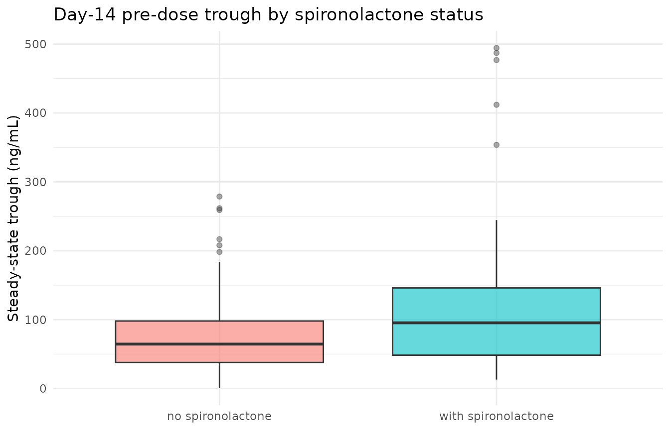
Simulated steady-state (day 14) whole-blood cyclosporin trough concentrations by spironolactone status, for a virtual cohort matched to the Wang 2019 Table I weight distribution and 25-80 mg/day dose range split q12h. Inter-individual variability is the published omega CL/F = 0.446 and omega V/F = 0.531; residual error is not applied to Cc.
trough_summary <- troughs |>
  dplyr::group_by(arm) |>
  dplyr::summarise(
    n = dplyr::n(),
    p10 = quantile(Cc, 0.10),
    median = median(Cc),
    p90 = quantile(Cc, 0.90),
    .groups = "drop"
  )

# These are cohort statistics, so assert on the centre and on robust
# quantiles, never on the extremes: the min/max of a random cohort is not
# reproducible across rxode2 versions or solver thread counts.
med_no <- trough_summary$median[trough_summary$arm == "no spironolactone"]
med_yes <- trough_summary$median[trough_summary$arm == "with spironolactone"]
stopifnot(
  nrow(trough_summary) == 2L,
  all(trough_summary$n == n_per_arm),
  all(troughs$Cc > 0),
  # A mis-transcribed CL/F, V/F, dose or unit moves the whole distribution by
  # tens of percent or more; this window is wide enough to survive a
  # different cohort draw and narrow enough to catch that.
  med_no > 20, med_no < 200,
  med_yes > 20, med_yes < 300,
  # Direction is a structural consequence of a -26.5% clearance effect on a
  # 100-subject arm, not a near-zero effect whose sign could flip.
  med_yes > med_no
)

trough_summary |>
  dplyr::rename(
    "Arm" = arm,
    "N" = n,
    "10th percentile (ng/mL)" = p10,
    "Median (ng/mL)" = median,
    "90th percentile (ng/mL)" = p90
  ) |>
  knitr::kable(
    digits = 1,
    caption = "Simulated day-14 steady-state trough distribution by spironolactone status."
)| Arm | N | 10th percentile (ng/mL) | Median (ng/mL) | 90th percentile (ng/mL) |
|---|---|---|---|---|
| no spironolactone | 100 | 23.2 | 64.5 | 139.2 |
| with spironolactone | 100 | 31.2 | 95.4 | 204.4 |
The median simulated trough is of the order of 60 ng/mL without
spironolactone and 110 ng/mL with it, with a 10th-to-90th-percentile
spread of roughly 20-220 ng/mL across the published 25-80 mg/day dose
range in a 10-23 kg child. That is the concentration window cyclosporin
TDM in pediatric nephrotic syndrome targets, and the spread is why the
doses in this study were titrated on trough rather than fixed. The model
reproducing the exposure regime that motivated the TDM programme is the
strongest available external check, because Wang 2019 publishes no NCA
table. Note that the trough spread here reflects only the published
inter-individual variability on CL/F and V/F plus the dose range; it
does not include residual error, which is applied to simulated
observations rather than to Cc.
Comparison against published non-compartmental results
Wang 2019 reports no Cmax / Tmax / AUC / half-life table: the dataset
was trough-only TDM, and the published validation is goodness-of-fit
plots (Fig. 2), a weighted-residual distribution (Fig. 3) and a
1,000-replicate bootstrap (Table III). There is therefore no published
NCA table to place side by side with the simulation, and
nlmixr2lib::ncaComparisonTable() is not used here. The
PKNCA block above instead validates the encoded model against its own
closed-form solution and against the dose-recovery identity, which is
the appropriate substitute.
The one published quantitative result that is independently checkable is the bootstrap column of Table III, reproduced below for reference. Every final estimate the model file encodes lies inside its own bootstrap 95% confidence interval, and the reported bias is under 1% for all parameters except V/F (15.3%) and the additive residual error (-7.1%) – the two parameters with the largest standard errors (75.4% and 32.6%).
tibble::tribble(
  ~Parameter, ~Estimate, ~SE_pct, ~Bootstrap_median, ~CI_low, ~CI_high, ~Bias_pct,
  "CL/F (L/h)", 80.7, 19.8, 79.900, 53.1, 106.5, -0.991,
  "V/F (L)", 2030, 75.4, 2340, 687, 3747.5, 15.271,
  "theta spironolactone", -0.265, 33.4, -0.266, -0.448, -0.066, 0.377,
  "omega CL/F", 0.446, 18.7, 0.445, 0.201, 0.569, -0.224,
  "omega V/F", 0.531, 30.1, 0.513, 0.005, 0.749, -3.390,
  "sigma1 (proportional)", 0.117, 18.4, 0.115, 0.047, 0.149, -1.710,
  "sigma2 (additive, ng/mL)", 8.062, 32.6, 7.490, 0.212, 11.843, -7.095
) |>
  dplyr::mutate(inside_ci = Estimate >= CI_low & Estimate <= CI_high) -> boot_tab

stopifnot(nrow(boot_tab) == 7L, all(boot_tab$inside_ci))

boot_tab |>
  dplyr::rename(
    "Parameter" = Parameter,
    "Estimate" = Estimate,
    "SE (%)" = SE_pct,
    "Bootstrap median" = Bootstrap_median,
    "95% CI lower" = CI_low,
    "95% CI upper" = CI_high,
    "Bias (%)" = Bias_pct,
    "Estimate inside CI" = inside_ci
  ) |>
  knitr::kable(
    digits = 3,
    caption = "Wang 2019 Table III, transcribed. Ka (0.68 1/h) is omitted because it was fixed and not bootstrapped."
)| Parameter | Estimate | SE (%) | Bootstrap median | 95% CI lower | 95% CI upper | Bias (%) | Estimate inside CI |
|---|---|---|---|---|---|---|---|
| CL/F (L/h) | 80.700 | 19.8 | 79.900 | 53.100 | 106.500 | -0.991 | TRUE |
| V/F (L) | 2030.000 | 75.4 | 2340.000 | 687.000 | 3747.500 | 15.271 | TRUE |
| theta spironolactone | -0.265 | 33.4 | -0.266 | -0.448 | -0.066 | 0.377 | TRUE |
| omega CL/F | 0.446 | 18.7 | 0.445 | 0.201 | 0.569 | -0.224 | TRUE |
| omega V/F | 0.531 | 30.1 | 0.513 | 0.005 | 0.749 | -3.390 | TRUE |
| sigma1 (proportional) | 0.117 | 18.4 | 0.115 | 0.047 | 0.149 | -1.710 | TRUE |
| sigma2 (additive, ng/mL) | 8.062 | 32.6 | 7.490 | 0.212 | 11.843 | -7.095 | TRUE |
Assumptions and deviations
Scale of the omega column (load-bearing). Wang 2019 Table III prints
omega CL/F = 0.446andomega V/F = 0.531, and the Abstract and Discussion quote the same two numbers as “the inter-individual variability in CL/F and V/F was 44.6 and 53.1%”. Those percentages are100 * omega, i.e. the small-omega approximationCV ~ omegaapplied to a standard deviation on the log scale. Reading the printed values as NONMEM$OMEGAvariances instead would giveCV = sqrt(0.446) = 66.8%andsqrt(0.531) = 72.9%, contradicting the paper’s own quoted percentages, and the exponential-model exact formsqrt(exp(omega^2) - 1)gives 46.9% and 57.0%, also not 44.6% and 53.1%. The printed column is therefore the standard deviation, and the model file encodesetalcl ~ 0.446^2andetalvc ~ 0.531^2. A supporting check: with n = 18 subjects the reported 18.7% relative standard error onomega CL/Fis close to the1/sqrt(2n) = 16.7%asymptotic RSE of a standard deviation and far from thesqrt(2/n) = 33%expected for a variance.Scale of the sigma column. Wang 2019 Table III prints
sigma1 = 0.117(“proportional error”) andsigma2 = 8.062(“additive error”) in the same column as the omega values, and the paper gives no separate residual CV%. They are taken on the same standard-deviation scale, sopropSd = 0.117(11.7%) andaddSd = 8.062ng/mL. Reading them as variances would give a 34.2% proportional error with a 2.84 ng/mL additive term, which is both inconsistent with the table’s omega convention and implausibly precise for whole-blood EMIT immunoassay TDM data. No check in this vignette depends on the residual error, which affects only simulated observations and notCc.Dosing interval assumed q12h. Wang 2019 Methods, ‘Drug administration’, states only “25-80 mg daily” and does not report the dosing interval. Cyclosporin is conventionally given twice daily, and the sibling pediatric model in this library (
Ni_2013_ciclosporin, the source of the fixedKa) used a BID schedule. The cohort simulation therefore splits the daily dose q12h. Because CL/F is linear, the steady-state average concentration is unaffected by the interval; only the peak-to-trough swing and hence the trough value depend on it. Users replicating a q24h schedule should expect lower troughs.No published NCA table. The study analysed only trough concentrations, so no Cmax / Tmax / AUC / half-life results exist in the source to compare against. The validation here is instead a closed-form identity check, a
CL/F * AUC = Dosemass-balance gate, and a transcription check of the Table III bootstrap. This is a deviation from the usual published-NCA comparison, not a gap in the model.No IIV on Ka.
Kawas fixed at 0.68 1/h and Wang 2019 Table III reports noomega Ka, so the model file carries noetalka. This is a direct consequence of the trough-only dataset: the absorption phase was never observed.-
Apparent (F-scaled) parameters. Wang 2019 Methods states explicitly that “it was not possible to estimate the bioavailability
- and absorption with a lag time”.
clandvcin the model file are therefore CL/F and V/F, and the whole dose entersdepot. TheCL/F * AUC = Dosegate above is exact for that reason; it would not be if an explicitf(depot)were applied.
- and absorption with a lag time”.
Extrapolation to the 70 kg reference. Every subject in the cohort weighed 10-23 kg, so the 70 kg reference values
CL/F = 80.7 L/handV/F = 2030 Lare extrapolations well outside the observed weight range and should not be read as adult estimates. At the cohort median of 15 kg the model gives CL/F = 25.4 L/h and V/F = 435 L, for a terminal half-life of 11.9 h without spironolactone and 16.1 h with it.Covariates screened but not retained. The Methods screened sex, age, height, albumin, globulin, albumin/globulin ratio, ALT, AST, creatinine, urea, total protein, total bile acid, direct and total bilirubin, hematocrit, hemoglobin, mean corpuscular hemoglobin, mean corpuscular hemoglobin concentration, and nine concomitant medications. Only body weight (pre-specified allometrically) and spironolactone survived. The screened terms are recorded in the model file’s
covariatesDataExcludedmetadata where a canonical covariate column exists, and inpopulation$notesotherwise (globulin, albumin/globulin ratio, mean corpuscular hemoglobin and its concentration have no canonical column and were not minted for a covariate with no retained effect).Unit of the urea column. Wang 2019 Table I prints urea as “Urea (umol/l)” with values 1.4-11.5. Blood urea is never at micromolar concentrations; the values are consistent with mmol/L and are recorded as mmol/L in
covariatesDataExcluded. Urea was not retained in the final model, so nothing in the encoded model depends on this.Spelling of the interacting drug. The paper writes “spirolactone” in its title, abstract, equations and Tables II-III. The rINN is spironolactone; the canonical covariate column is
CONMED_SPIRON, withspirolactonerecorded as a source alias ininst/references/covariate-columns.md.Form of the covariate equation. The Abstract prints
CL/F = 80.7 x (WT/70)^0.75 x (1 - 0.265 x theta_spirolactone), which conflates the indicator with its coefficient. The Results section prints the well-formed generic version,CL/F = theta_CL/F x (WT/70)^0.75 x (1 + spirolactone x theta_spirolactone)with the indicator 1/0 andtheta_spirolactone = -0.265. The model file encodes the Results form. Both evaluate to the same number (80.7 x 0.735with spironolactone), so nothing turns on the choice.No inter-occasion variability. Wang 2019 reports no IOV term, and the retrospective TDM dataset had no occasion structure, so none is encoded.