Vancomycin in infants by renal function (Li 2021)

Model and source

Li 2021 developed three population PK models of vancomycin in parallel from one retrospective cohort of Chinese infants aged 1-24 months. The cohort was split by renal function (modified-Schwartz eGFR):

Paper label	nlmixr2lib model	Group	Covariates
Model 1	`Li_2021_vancomycin_normal`	normal renal function, eGFR 30-86 mL/min/1.73 m^2	WT on CL and V; SCR on CL
Model 2	`Li_2021_vancomycin_arc`	augmented renal clearance (ARC), eGFR >= 86 mL/min/1.73 m^2	WT on CL and V
Model 3	`Li_2021_vancomycin_all`	all infants with eGFR >= 30 mL/min/1.73 m^2 (pooled)	WT on CL and V; SCR on CL

Citation: Li DY, Li L, Li GZ, Hu YH, Guo HL, Jing X, Chen F, Ji X, Xu J, Dai HR. Population Pharmacokinetics Modeling of Vancomycin Among Chinese Infants With Normal and Augmented Renal Function. Front Pediatr. 2021;9:713588. doi:10.3389/fped.2021.713588
Article: Front Pediatr 2021;9:713588

Descriptions:

Model 1: One-compartment IV-infusion population PK model for vancomycin in Chinese infants (1-24 months) with normal renal function, eGFR 30-86 mL/min/1.73 m^2 (Li 2021, Model 1). CL scales as a power of body weight (reference 2.25 kg, estimated exponent 1.24) and exponentially with serum creatinine (exp(-0.533 * SCR / 27.1)); V scales as a power of body weight (reference 2.25 kg, estimated exponent 1.28). IIV on CL only; proportional residual error.
Model 2: One-compartment IV-infusion population PK model for vancomycin in Chinese infants (1-24 months) with augmented renal clearance, eGFR >= 86 mL/min/1.73 m^2 (Li 2021, Model 2). Body weight is the only covariate: CL and V scale as powers of body weight (reference 4.6 kg, estimated exponents 1.03 and 0.918). IIV on CL only; proportional residual error.
Model 3: One-compartment IV-infusion population PK model for vancomycin in Chinese infants (1-24 months) across all levels of renal function, eGFR >= 30 mL/min/1.73 m^2 (Li 2021, Model 3, pooled). CL scales as a power of body weight (reference 3.45 kg, estimated exponent 1.23) and exponentially with serum creatinine (exp(-0.377 * SCR / 19)); V scales as a power of body weight (reference 3.45 kg, estimated exponent 1.29). IIV on CL only; proportional residual error.

Population

Infants aged 1-24 months who received IV vancomycin for at least 3 days at the Children’s Hospital of Nanjing Medical University between January 2017 and July 2021 were enrolled (Li 2021 Methods “Patients”). Each had at least one trough and one peak concentration, and an eGFR of at least 30 mL/min/1.73 m^2. Vancomycin was given as an IV infusion lasting at least 60 min, two to four times daily, with doses adjusted by therapeutic drug monitoring. Whole-blood samples were drawn 30 min before the fifth dose (trough) and 30 min after the fifth dose (peak), and assayed by EMIT.

Li 2021 Table 2 summarises the three modelling groups:

	Model 1 (normal)	Model 2 (ARC)	Model 3 (all)
Patients (male/female)	61 (37/24)	64 (41/23)	115 (73/42)
Concentrations (trough/peak)	135 (69/66)	139 (88/51)	276 (158/118)
Preterm infants	29	17	46
Weight, kg, median (range)	2.25 (1.15-13)	4.60 (2.2-14)	3.3 (1.15-14)
SCR, umol/L, median (range)	27.1 (14-315)	16.8 (8-29)	18.95 (8-147)
eGFR, mL/min/1.73 m^2, median (range)	57.56 (30-85.56)	128 (90.8-280)	98.7 (30-280)
Daily dose, mg/day, median (range)	75 (24-320)	216 (50-640)	145 (24-640)
Trough, mg/L, median (range)	7.05 (2.1-22.2)	7 (2.1-23)	7.1 (2.1-23)
Peak, mg/L, median (range)	19.9 (6.8-46.9)	18.7 (6.1-36.6)	19.1 (6.1-46.9)

The Model 1 and Model 2 group sizes add up to more than 115. Patients whose renal function changed during treatment were counted in both groups (Results “Patients”). The same information is available programmatically, for example readModelDb("Li_2021_vancomycin_normal")()$population.

Source trace

Each model has the same structure: a one-compartment model with first-order elimination (NONMEM ADVAN1 TRANS2), exponential IIV on CL only, and a proportional residual error. The covariate equations are printed both as the header row of Tables 5-7 and as the three final-model equations in Results “Model Building”:

Model 1: CL = theta1 * (WT/2.25)^theta3 * exp(theta5 * SCR/27.1); V = theta2 * (WT/2.25)^theta4
Model 2: CL = theta1 * (WT/4.6)^theta3; V = theta2 * (WT/4.6)^theta4
Model 3: CL = theta1 * (WT/3.45)^theta3 * exp(theta5 * SCR/19); V = theta2 * (WT/3.45)^theta4

Parameter	Model 1	Model 2	Model 3	Source
`lcl` (theta1, L/h)	log(0.407)	log(0.756)	log(0.707)	Tables 5 / 6 / 7
`lvc` (theta2, L)	log(1.86)	log(4.89)	log(3.39)	Tables 5 / 6 / 7
`e_wt_cl` (theta3)	1.24	1.03	1.23	Tables 5 / 6 / 7
`e_wt_vc` (theta4)	1.28	0.918	1.29	Tables 5 / 6 / 7
`e_creat_cl` (theta5)	-0.533	n/a	-0.377	Tables 5 / 7
`etalcl` (BSV_CL squared)	0.315^2	0.312^2	0.311^2	Tables 5 / 6 / 7
`propSd` (PROP_RV)	0.319	0.319	0.335	Tables 5 / 6 / 7
WT reference (kg)	2.25	4.6	3.45	Table header equations; Results equations
SCR divisor (umol/L)	27.1	n/a	19	Table header equations; Results equations
1-cmt, first-order elimination				Methods “Base Model”
Exponential IIV				Methods “Base Model”
Proportional residual `Y = F*(1+eps)`				Methods “Base Model”; PROP_RV row

Scale of `BSV_CL` and `PROP_RV`

Li 2021 does not say whether BSV_CL and PROP_RV are standard deviations or variances. The footnotes call PROP_RV a “proportional residual variance”, which suggests a variance. The observed peak concentrations rule that reading out.

A peak sampled 30 min after the infusion carries the full proportional residual error. The coefficient of variation (CV) of observed peaks therefore cannot be smaller than the residual SD. If PROP_RV were a variance, the residual SD would be sqrt(0.319) = 0.565. Yet the peaks in every group of Table 2 vary with a CV of only 36-39%, even though that CV also includes between-subject, covariate and dose variation. So PROP_RV must be an SD. The same table reports BSV_CL on the same scale, so it is also read as the SD of eta, and its square gives the variance used in ini().

scale_check <- tibble::tribble(
  ~model,    ~prop_rv, ~peak_mean, ~peak_sd,
  "Model 1", 0.319,    22.28,      8.75,
  "Model 2", 0.319,    18.82,      6.76,
  "Model 3", 0.335,    20.61,      7.67
) |>
  mutate(
    observed_peak_cv = peak_sd / peak_mean,
    residual_sd_if_variance = sqrt(prop_rv),
    residual_sd_if_sd = prop_rv
  )

# Table 2 arithmetic, no simulation. The variance reading would need an
# observed peak CV of at least sqrt(PROP_RV) = 0.565-0.579; observed is
# 0.36-0.39. The SD reading (0.319-0.335) sits below it, as it must.
stopifnot(
  all(scale_check$observed_peak_cv < scale_check$residual_sd_if_variance),
  all(scale_check$observed_peak_cv > scale_check$residual_sd_if_sd)
)

scale_check |>
  dplyr::rename(
    "Model" = model,
    "PROP_RV (Tables 5-7)" = prop_rv,
    "Observed peak CV (Table 2)" = observed_peak_cv,
    "Residual SD if variance" = residual_sd_if_variance,
    "Residual SD if SD" = residual_sd_if_sd
  ) |>
  dplyr::select(-peak_mean, -peak_sd) |>
  knitr::kable(digits = 3, caption = "Observed peak variability versus the two readings of PROP_RV.")

Observed peak variability versus the two readings of PROP_RV.
Model	PROP_RV (Tables 5-7)	Observed peak CV (Table 2)	Residual SD if variance	Residual SD if SD
Model 1	0.319	0.393	0.565	0.319
Model 2	0.319	0.359	0.565	0.319
Model 3	0.335	0.372	0.579	0.335

Typical-value check against the observed troughs and peaks

Li 2021 reports no NCA table, and its VPCs (Figures 4-6) are plotted against time since the first dose, pooled across dose levels. The most direct check of the printed equations uses the observed median troughs and peaks in Table 2. The typical infant of each group is given the Table 2 median weight and SCR. That infant receives the Table 2 median daily dose as 1-h infusions every 8 h. The trough is read 30 min before the fifth dose and the peak 30 min after the fifth infusion ends, which matches the sampling design.

These are typical-value predictions compared with population medians, not identical quantities. The check is still sharp on the covariate equations. The creatinine factor is not centred: at the reference SCR, exp(theta5) is 0.59 for Model 1 and 0.69 for Model 3. Dropping it, or re-centring it as exp(theta5 * (SCR/27.1 - 1)), puts the Model 1 typical trough 50% and its peak 34% below the observed medians, so both gates below would fail.

typical_cases <- tibble::tribble(
  ~model,                        ~label,    ~WT,  ~CREAT, ~daily_dose, ~obs_trough, ~obs_peak,
  "Li_2021_vancomycin_normal",   "Model 1", 2.25, 27.1,   75,          7.05,        19.9,
  "Li_2021_vancomycin_arc",      "Model 2", 4.60, 16.8,   216,         7.0,         18.7,
  "Li_2021_vancomycin_all",      "Model 3", 3.3,  18.95,  145,         7.1,         19.1
)

tau <- 8
tinf <- 1
n_dose <- 5
dose_times <- seq(0, by = tau, length.out = n_dose)
t_trough <- dose_times[n_dose] - 0.5
t_peak <- dose_times[n_dose] + tinf + 0.5

typical_one <- function(i) {
  case <- typical_cases[i, ]
  amt <- case$daily_dose * tau / 24
  ev <- dplyr::bind_rows(
    tibble(time = dose_times, evid = 1L, amt = amt, rate = amt / tinf),
    tibble(time = c(t_trough, t_peak), evid = 0L, amt = 0, rate = 0)
  ) |>
    mutate(id = 1L, cmt = "central", WT = case$WT, CREAT = case$CREAT) |>
    arrange(time, desc(evid))
  mod_typ <- rxode2::zeroRe(readModelDb(case$model))
  s <- as.data.frame(rxode2::rxSolve(mod_typ, events = ev, rtol = 1e-10, atol = 1e-12))
  tibble(
    label = case$label,
    pred_trough = s$Cc[s$time == t_trough],
    pred_peak = s$Cc[s$time == t_peak]
  )
}

typical_res <- dplyr::bind_rows(lapply(seq_len(nrow(typical_cases)), typical_one)) |>
  left_join(dplyr::select(typical_cases, label, obs_trough, obs_peak), by = "label") |>
  mutate(
    trough_pct = 100 * (pred_trough / obs_trough - 1),
    peak_pct = 100 * (pred_peak / obs_peak - 1)
  )
#> ℹ parameter labels from comments will be replaced by 'label()'
#> ℹ omega/sigma items treated as zero: 'etalcl'
#> ℹ parameter labels from comments will be replaced by 'label()'
#> ℹ omega/sigma items treated as zero: 'etalcl'
#> ℹ parameter labels from comments will be replaced by 'label()'
#> ℹ omega/sigma items treated as zero: 'etalcl'

# Deterministic (zeroRe, one subject per model). Measured: trough +19 / -0 /
# +13 %, peak -8 / -5 / +0 % for Models 1 / 2 / 3. A dropped or re-centred
# creatinine factor gives -50 % (trough) and -34 % (peak) for Model 1; a dose
# or volume mis-transcription moves the peaks by tens of percent.
stopifnot(
  nrow(typical_res) == 3L,
  all(abs(typical_res$trough_pct) < 30),
  all(abs(typical_res$peak_pct) < 20)
)

typical_res |>
  dplyr::rename(
    "Model" = label,
    "Predicted trough (mg/L)" = pred_trough,
    "Observed median trough (mg/L)" = obs_trough,
    "Trough difference (%)" = trough_pct,
    "Predicted peak (mg/L)" = pred_peak,
    "Observed median peak (mg/L)" = obs_peak,
    "Peak difference (%)" = peak_pct
  ) |>
  knitr::kable(digits = 2, caption = "Typical-infant trough and peak around the fifth dose (median daily dose, q8h, 1-h infusion) versus the Table 2 observed medians.")

Typical-infant trough and peak around the fifth dose (median daily dose, q8h, 1-h infusion) versus the Table 2 observed medians.
Model	Predicted trough (mg/L)	Predicted peak (mg/L)	Observed median trough (mg/L)	Observed median peak (mg/L)	Trough difference (%)	Peak difference (%)
Model 1	8.39	18.32	7.05	19.9	18.96	-7.96
Model 2	6.99	17.76	7.00	18.7	-0.19	-5.05
Model 3	8.02	19.11	7.10	19.1	12.93	0.04

Virtual cohort

The original data are not public. Each model gets its own virtual cohort of 200 infants, drawn to resemble its Table 2 group. Weight and SCR are log-normal. The median is the Table 2 median, and the log-SD is set so the distribution also reproduces the Table 2 mean (sdlog = sqrt(2 * log(mean / median))). Values outside the Table 2 range are redrawn. Every infant gets the group’s median daily dose per kg (Table 2 median daily dose divided by median weight) as 1-h infusions every 8 h, for 12 doses.

rxode2::rxSetSeed(20210920)
set.seed(20210920)

n_per_arm <- 200L
n_dose_sim <- 12L
dose_times_sim <- seq(0, by = tau, length.out = n_dose_sim)

# Reject-and-redraw inside [lo, hi]; clamping would pile subjects on the bounds.
rlnorm_range <- function(n, median, mean, lo, hi) {
  sdlog <- sqrt(2 * log(mean / median))
  out <- numeric(0)
  while (length(out) < n) {
    x <- stats::rlnorm(4 * n, log(median), sdlog)
    out <- c(out, x[x >= lo & x <= hi])
  }
  out[seq_len(n)]
}

arms <- tibble::tribble(
  ~model,                      ~label,    ~wt_med, ~wt_mean, ~wt_lo, ~wt_hi, ~cr_med, ~cr_mean, ~cr_lo, ~cr_hi, ~dd_med,
  "Li_2021_vancomycin_normal", "Model 1", 2.25,    2.86,     1.15,   13,     27.1,    30.80,    14,     315,    75,
  "Li_2021_vancomycin_arc",    "Model 2", 4.60,    5.34,     2.2,    14,     16.8,    16.84,    8,      29,     216,
  "Li_2021_vancomycin_all",    "Model 3", 3.3,     4.11,     1.15,   14,     18.95,   23.54,    8,      147,    145
)

obs_times <- sort(unique(c(
  seq(0, max(dose_times_sim) + tau, by = 0.5),
  t_trough, t_peak
)))

make_arm <- function(i) {
  a <- arms[i, ]
  subj <- tibble(
    id = (i - 1L) * n_per_arm + seq_len(n_per_arm),
    WT = rlnorm_range(n_per_arm, a$wt_med, a$wt_mean, a$wt_lo, a$wt_hi),
    # Model 2 has no creatinine term; SCR is drawn for every arm so the
    # event tables share one shape (its Table 2 mean ~ median gives a
    # near-degenerate spread, which is harmless there).
    CREAT = rlnorm_range(n_per_arm, a$cr_med, max(a$cr_mean, a$cr_med * 1.001), a$cr_lo, a$cr_hi),
    mgkg_day = a$dd_med / a$wt_med
  ) |>
    mutate(amt = mgkg_day * WT * tau / 24)
  doses <- tidyr::expand_grid(id = subj$id, time = dose_times_sim) |>
    left_join(dplyr::select(subj, id, amt), by = "id") |>
    mutate(evid = 1L, rate = amt / tinf)
  obs <- tidyr::expand_grid(id = subj$id, time = obs_times) |>
    mutate(evid = 0L, amt = 0, rate = 0)
  dplyr::bind_rows(doses, obs) |>
    left_join(dplyr::select(subj, id, WT, CREAT), by = "id") |>
    mutate(cmt = "central", model = a$model, label = a$label) |>
    arrange(id, time, desc(evid))
}

events_all <- dplyr::bind_rows(lapply(seq_len(nrow(arms)), make_arm))
stopifnot(!anyDuplicated(unique(events_all[, c("id", "time", "evid")])))

Simulation

sim <- dplyr::bind_rows(lapply(seq_len(nrow(arms)), function(i) {
  ev <- dplyr::filter(events_all, model == arms$model[i])
  rxode2::rxSolve(
    readModelDb(arms$model[i]),
    events = ev,
    keep = c("label", "WT", "CREAT")
  ) |>
    as.data.frame()
}))
#> ℹ parameter labels from comments will be replaced by 'label()'
#> ℹ parameter labels from comments will be replaced by 'label()'
#> ℹ parameter labels from comments will be replaced by 'label()'

Replicate published figures

Figures 4-6 of Li 2021 are VPCs of observed concentrations against time since the first dose. The patients were sampled around their fifth dose, and their treatment courses ran for different lengths. The plot below shows the same quantity for the virtual cohorts: the median and 90% prediction interval of simulated whole-blood concentrations (with residual error). The dashed lines mark the Table 2 observed median trough and peak.

obs_lines <- tibble::tribble(
  ~label,    ~trough, ~peak,
  "Model 1", 7.05,    19.9,
  "Model 2", 7.0,     18.7,
  "Model 3", 7.1,     19.1
) |>
  tidyr::pivot_longer(c(trough, peak), names_to = "sample", values_to = "conc")

sim |>
  group_by(label, time) |>
  summarise(
    Q05 = quantile(sim, 0.05, na.rm = TRUE),
    Q50 = quantile(sim, 0.50, na.rm = TRUE),
    Q95 = quantile(sim, 0.95, na.rm = TRUE),
    .groups = "drop"
  ) |>
  ggplot(aes(time, Q50)) +
  geom_ribbon(aes(ymin = Q05, ymax = Q95), alpha = 0.25, fill = "steelblue") +
  geom_line(colour = "firebrick") +
  geom_hline(data = obs_lines, aes(yintercept = conc, linetype = sample)) +
  facet_wrap(~label, ncol = 1) +
  labs(
    x = "Time since first dose (h)", y = "Vancomycin (mg/L)", linetype = "Table 2 median",
    title = "Simulated concentrations, median and 90% PI",
    caption = "Compare with Figures 4-6 of Li 2021 (VPCs of Models 1-3)."
  )

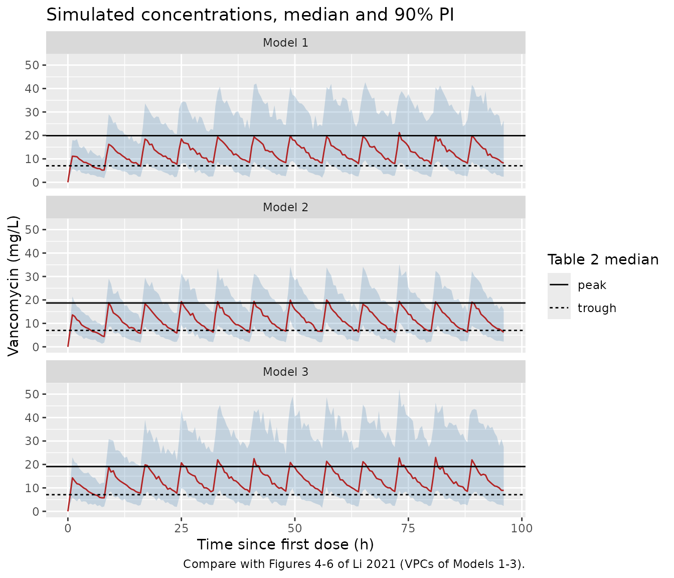
Simulated troughs and peaks around the fifth dose, with residual error, compared with the Table 2 observed medians and ranges. The simulated CVs are larger than the observed ones. In the study, doses were adjusted by drug monitoring, which narrows the observed spread, and the virtual cohort draws some infants from the high-creatinine tail. The comparison does not favour the variance reading of BSV_CL and PROP_RV. That reading would widen the simulated spread further.

fifth <- sim |>
  filter(time %in% c(t_trough, t_peak)) |>
  mutate(sample = ifelse(time == t_trough, "trough", "peak")) |>
  group_by(label, sample) |>
  summarise(
    sim_median = median(sim),
    sim_p05 = quantile(sim, 0.05),
    sim_p95 = quantile(sim, 0.95),
    sim_cv = sd(sim) / mean(sim),
    .groups = "drop"
  ) |>
  left_join(
    tibble::tribble(
      ~label,    ~sample,  ~obs_median, ~obs_range,  ~obs_cv,
      "Model 1", "trough", 7.05,        "2.1-22.2",  4.67 / 8.29,
      "Model 1", "peak",   19.9,        "6.8-46.9",  8.75 / 22.28,
      "Model 2", "trough", 7.0,         "2.1-23",    4.66 / 7.93,
      "Model 2", "peak",   18.7,        "6.1-36.6",  6.76 / 18.82,
      "Model 3", "trough", 7.1,         "2.1-23",    4.75 / 8.31,
      "Model 3", "peak",   19.1,        "6.1-46.9",  7.67 / 20.61
    ),
    by = c("label", "sample")
  )

# Cohort medians against observed medians. The observed doses were TDM-adjusted
# and varied per infant, so the check is on the centre with a wide envelope.
# Measured simulated/observed median ratios: 0.89-1.27 across the six cells.
# The deterministic typical-value check above is the sharp structural gate;
# this one catches unit or dose errors, which move the medians several-fold.
stopifnot(
  nrow(fifth) == 6L,
  all(fifth$sim_median / fifth$obs_median > 0.6),
  all(fifth$sim_median / fifth$obs_median < 1.6)
)

fifth |>
  dplyr::rename(
    "Model" = label, "Sample" = sample,
    "Simulated median" = sim_median, "Simulated 5th pct" = sim_p05,
    "Simulated 95th pct" = sim_p95, "Simulated CV" = sim_cv,
    "Observed median" = obs_median, "Observed range" = obs_range,
    "Observed CV" = obs_cv
  ) |>
  knitr::kable(digits = 2, caption = "Troughs (30 min before the fifth dose) and peaks (30 min after the fifth infusion), simulated versus Li 2021 Table 2 (mg/L).")

Troughs (30 min before the fifth dose) and peaks (30 min after the fifth infusion), simulated versus Li 2021 Table 2 (mg/L).
Model	Sample	Simulated median	Simulated 5th pct	Simulated 95th pct	Simulated CV	Observed median	Observed range	Observed CV
Model 1	peak	18.25	7.42	40.82	0.50	19.90	6.8-46.9	0.39
Model 1	trough	8.95	2.50	22.72	0.62	7.05	2.1-22.2	0.56
Model 2	peak	16.62	8.30	28.20	0.38	18.70	6.1-36.6	0.36
Model 2	trough	6.87	2.20	15.27	0.55	7.00	2.1-23	0.59
Model 3	peak	20.21	9.02	45.36	0.52	19.10	6.1-46.9	0.37
Model 3	trough	8.34	2.68	25.48	0.77	7.10	2.1-23	0.57

PKNCA validation

Steady-state NCA over the 12th dosing interval, grouped by model. At steady state, the AUC over one dosing interval equals the dose divided by the individual CL. The check below compares the two for each virtual infant.

t_start <- max(dose_times_sim)
t_end <- t_start + tau

sim_nca <- sim |>
  filter(!is.na(Cc), time >= t_start, time <= t_end) |>
  mutate(Cc = pmax(Cc, 0)) |>
  dplyr::select(id, time, Cc, label)

dose_nca <- events_all |>
  filter(evid == 1, time == t_start) |>
  dplyr::select(id, time, amt, label)

conc_obj <- PKNCA::PKNCAconc(sim_nca, Cc ~ time | label + id, concu = "mg/L", timeu = "h")
dose_obj <- PKNCA::PKNCAdose(dose_nca, amt ~ time | label + id, doseu = "mg")
intervals <- data.frame(
  start = t_start, end = t_end,
  cmax = TRUE, cmin = TRUE, tmax = TRUE, auclast = TRUE, cav = TRUE
)
nca_res <- PKNCA::pk.nca(PKNCA::PKNCAdata(conc_obj, dose_obj, intervals = intervals))

knitr::kable(summary(nca_res), caption = "Simulated steady-state NCA (12th dosing interval, q8h) by model.")

Simulated steady-state NCA (12th dosing interval, q8h) by model.
Interval Start	Interval End	label	N	AUClast (h*mg/L)	Cmax (mg/L)	Cmin (mg/L)	Tmax (h)	Cav (mg/L)
88	96	Model 1	200	112 [45.4]	20.6 [31.9]	8.73 [69.2]	1.00 [1.00, 1.00]	14.0 [45.4]
88	96	Model 2	200	97.0 [31.0]	19.8 [17.7]	6.45 [56.8]	1.00 [1.00, 1.00]	12.1 [31.0]
88	96	Model 3	200	120 [49.2]	22.8 [34.6]	8.91 [75.7]	1.00 [1.00, 1.00]	15.0 [49.2]


auc_check <- as.data.frame(nca_res) |>
  filter(PPTESTCD == "auclast") |>
  dplyr::select(id, label, auclast = PPORRES) |>
  left_join(
    sim |> filter(time == t_start) |> dplyr::select(id, cl),
    by = "id"
  ) |>
  left_join(dplyr::select(dose_nca, id, amt), by = "id") |>
  mutate(pct_diff = 100 * (auclast * cl / amt - 1))

# AUCtau * CL_i / Dose = 1 at steady state. Deviations come from the
# 0.5-h trapezoid grid and from the slowest-clearing infants not being fully
# at steady state after 88 h. Measured: median -0.04 %, 90th percentile of
# |difference| 0.09-0.21 % per model; the bounds leave room for a cohort with
# more slow-clearing infants while still failing on any dose or CL error.
stopifnot(
  nrow(auc_check) == 3L * n_per_arm,
  abs(median(auc_check$pct_diff)) < 1,
  quantile(abs(auc_check$pct_diff), 0.9) < 5
)

auc_check |>
  group_by(label) |>
  summarise(
    median_pct_diff = median(pct_diff),
    p90_abs_pct_diff = quantile(abs(pct_diff), 0.9),
    .groups = "drop"
  ) |>
  dplyr::rename(
    "Model" = label,
    "Median (AUCtau*CL/Dose - 1), %" = median_pct_diff,
    "90th pct of |difference|, %" = p90_abs_pct_diff
  ) |>
  knitr::kable(digits = 2, caption = "Steady-state AUCtau against Dose / individual CL.")

Steady-state AUCtau against Dose / individual CL.
Model	Median (AUCtau*CL/Dose - 1), %	90th pct of \|difference\|, %
Model 1	-0.04	0.21
Model 2	-0.04	0.09
Model 3	-0.04	0.13

Li 2021 reports no NCA parameters, so there is no published NCA table to compare against. The comparison with the paper is the trough and peak check above.

Assumptions and deviations

IIV and residual-error scale. Tables 5-7 do not say whether BSV_CL and PROP_RV are SDs or variances, and the footnote calls PROP_RV a “variance”. The maintainers read both as SDs. As shown in the “Scale of BSV_CL and PROP_RV” section, the variance reading needs a residual SD of 0.565-0.579, which is larger than the observed peak CV of 0.36-0.39 in every group. etalcl is therefore BSV_CL^2 and propSd is PROP_RV.
Uncentred creatinine factor. The creatinine term is encoded exactly as printed, exp(theta5 * SCR / 27.1) (Model 1) and exp(theta5 * SCR / 19) (Model 3), in both the Table 5/7 header equations and the Results equations. It equals exp(theta5), not 1, at the reference SCR, so exp(lcl) is not the typical CL of the reference infant. The as-printed form is the one that reproduces the observed troughs and peaks (typical-value check above).
Model 3 weight reference. The Model 3 equations divide weight by 3.45 kg, while Table 2 gives a median of 3.3 kg for that group. The printed equation value (3.45 kg) is used. The Model 3 SCR divisor (19 umol/L) matches the Table 2 median of 18.95 umol/L after rounding.
Group labels. Table 2’s column headers call the Model 1 group “reduced renal function” and the Model 2 group “normal renal function”. The abstract, Methods and Results call them the normal-renal-function and ARC groups. The model names follow the abstract, Methods and Results.
Dosing in the vignette. The paper gives the daily dose (Table 2) and says infusions last at least 60 min and are given two to four times daily. The vignette uses 1-h infusions every 8 h at each group’s median mg/kg/day. “30 min after the fifth administration” is read as 30 min after the end of the fifth infusion.
Covariate distributions. Weight and SCR are drawn independently. The paper does not report their correlation.
Covariates not retained. Sex, age, height, ALT, AST, BUN, cystatin C, albumin, total protein, eGFR, and meropenem or imipenem co-administration were screened (Table 4 for Model 1) but are not in any final model. eGFR defines which model applies (Model 1: 30-86; Model 2: >= 86 mL/min/1.73 m^2) but is not a model covariate.
Specimen. Li 2021 assayed whole blood (Methods “Bioassay”), so the concentrations are whole-blood vancomycin concentrations.
Errata. No correction notice for this article was found on Crossref as of 2026-09-29.