Leuprolide testosterone suppression in normal and prostate-cancer rats (Lee 2018)
Source:vignettes/articles/Lee_2018_leuprolide.Rmd
Lee_2018_leuprolide.RmdModel and source
Lee 2018 fits one PK-PD structure to four separate experimental groups of a six-group rat study, so the paper contributes four model files. All four share the testosterone feedback-turnover PD model; they differ in the leuprolide input (intravenous bolus, subcutaneous solution, or a three-section sustained-release microsphere depot) and in the strain / disease state.
model_names <- c(
  "Lee_2018_leuprolide_iv_rat",
  "Lee_2018_leuprolide_sc_rat",
  "Lee_2018_leuprolide_sr_rat",
  "Lee_2018_leuprolide_sr_cancer_rat"
)
uis <- lapply(model_names, function(n) rxode2::rxode(readModelDb(n)))
names(uis) <- model_names

tibble::tibble(
  Model = model_names,
  Group = c(
    "Group 1 - Wistar, IV leuprolide solution",
    "Group 3 - Wistar, SC leuprolide solution",
    "Group 4 - Wistar, SC Lucrin sustained-release depot",
    "Group 6 - Iar:COP (prostate cancer), SC Lucrin sustained-release depot"
  ),
  Species = vapply(uis, function(u) u$population$species, character(1))
) |>
knitr::kable(caption = "The four models this paper contributes.")| Model | Group | Species |
|---|---|---|
| Lee_2018_leuprolide_iv_rat | Group 1 - Wistar, IV leuprolide solution | rat (Wistar) |
| Lee_2018_leuprolide_sc_rat | Group 3 - Wistar, SC leuprolide solution | rat (Wistar) |
| Lee_2018_leuprolide_sr_rat | Group 4 - Wistar, SC Lucrin sustained-release depot | rat (Wistar) |
| Lee_2018_leuprolide_sr_cancer_rat | Group 6 - Iar:COP (prostate cancer), SC Lucrin sustained-release depot | rat (Iar:COP, Copenhagen) |
- Citation: Lee DS, Kim SJ, Choi GW, Lee YB, Cho HY. Pharmacokinetic-Pharmacodynamic Model for the Testosterone-Suppressive Effect of Leuprolide in Normal and Prostate Cancer Rats. Molecules. 2018;23(4):909. doi:10.3390/molecules23040909
- Article: https://doi.org/10.3390/molecules23040909
- PubMed Central: https://www.ncbi.nlm.nih.gov/pmc/articles/PMC6017563/
The paper is open access; the 16 numbered display equations were read from the publisher’s MathML rather than from the PDF text layer, and Figures 2, 3 and 5 were read from the publisher’s figure files at native resolution.
Population
Adult male rats, n = 5 per group, in six groups (Methods
4.3 and Table 5). Normal animals were Wistar; the prostate-cancer
animals were Iar:COP (Copenhagen) rats carrying spontaneous Dunning
R-3327 prostate adenocarcinoma. Each animal received a single dose of
0.1 mg/kg leuprolide acetate - as a solution intravenously (Group 1) or
subcutaneously (Group 3), or as a Lucrin depot microsphere dispersion
subcutaneously (Groups 4 and 6) - or the dispersion vehicle alone
(Groups 2 and 5, which supplied the drug-free testosterone baseline).
Blood was sampled pre-dose and at 0.25, 1, 2, 4 and 8 h and at 1, 2, 3,
4, 5, 6, 7, 11 and 14 days. Leuprolide was assayed by UPLC-MS/MS and
testosterone by a competitive ELISA linear over 0.041-10 ng/mL (Methods
4.4, 4.5).
The same information is available programmatically from each model’s
population metadata, e.g.
rxode2::rxode(readModelDb("Lee_2018_leuprolide_iv_rat"))$population.
Body weight and the administered amount
Body weight is not reported anywhere in the paper, so the 0.1 mg/kg dose cannot be converted to an amount directly. The paper’s own definition of clearance (Methods 4.6: “The clearance (CL) was calculated as the dose of leuprolide divided by AUC0-inf”) back-solves it from Table 1, once per route:
dose_iv <- 105.50 * 248.61 # AUC0-inf (h*ng/mL) x CL (mL/h), Table 1 IV column
dose_sc <- 53.33 * 514.46 # AUC0-inf (h*ng/mL) x CL/F (mL/h), Table 1 SC column
c(dose_iv_ng = dose_iv, dose_sc_ng = dose_sc, implied_bw_g_iv = dose_iv / 100, implied_bw_g_sc = dose_sc / 100)
#>      dose_iv_ng      dose_sc_ng implied_bw_g_iv implied_bw_g_sc
#>      26228.3550      27436.1518        262.2836        274.3615
The two routes are independent arithmetic on different table columns yet imply body weights of 262 g and 274 g - 4.5% apart, and both squarely in the normal range for an adult male rat. That agreement is the reason these amounts are used below rather than an assumed weight. The depot groups received “0.1 mg/kg (as leuprolide)” (Table 5) and are given the subcutaneous amount.
Source trace
Per-parameter provenance is recorded as an in-file comment beside
each ini() entry in the four files under
inst/modeldb/specificDrugs/. Collected here:
| Equation / parameter | Value(s) | Source location |
|---|---|---|
d/dt(depot), d/dt(central),
Cc (solution) |
n/a | Equations (1), (2), (3) |
d/dt(depot), d/dt(depot2),
d/dt(transit1), d/dt(transit2),
d/dt(central), Cc (depot) |
n/a | Equations (4), (5), (6), (8), (9), (10) |
frel + frel2 + frel3 == 1 |
n/a | Equation (7) |
d/dt(TT) baseline form |
n/a | Equation (11) |
TT(0) <- rbase_tt |
4.353 (Wistar), 4.094 (Iar:COP) | Equations (12), (13) |
d/dt(TT) drug-effect form |
n/a | Equation (14) |
d/dt(moderator1) |
n/a | Equation (15) |
ce sigmoid Emax |
n/a | Equation (16) |
lka |
16.67 1/h | Table 1, SC (Group 3), row k a
|
lcl |
248.61 mL/h (IV); 514.46 mL/h (SC and both depots) | Table 1, row CL
|
lvc |
192.95 mL (IV); 487.40 mL (SC and both depots) | Table 1, row V d
|
lka2 (paper’s kd) |
0.08 1/h both strains | Table 2, row k d
|
lktr (paper’s kt) |
0.0078 1/h (Wistar); 0.0193 1/h (Iar:COP) | Table 2, row k t
|
logitfrel, logitfrel2 (paper’s
NR, DR, ER) |
0.18 / 0.28 / 0.54 (Wistar); 0.08 / 0.43 / 0.49 (Iar:COP) | Table 2, rows N R, D R,
E R
|
ltlag, ltlag2
|
0.47 / 3.61 h (Wistar); 0.35 / 2.58 h (Iar:COP) | Table 2, rows t lag,d, t lag ,e
|
| erosion chain length = 2 | 2 (fixed) | Table 2, row ES n; Results 2.4 |
lkin_tt, lkout_tt
|
0.68 / 0.16 (Wistar); 0.35 / 0.06 (Iar:COP) | Table 4, rows k in, k out
|
lhill |
2.00 / 2.02 / 2.00 / 3.18 | Table 4, row h
|
lemax |
303.77 / 183.50 / 380.00 / 634.50 | Table 4, row E max
|
lec50 |
3.48 / 6.17 / 1.80 / 3.34 ng/mL | Table 4, row EC 50
|
lkin_moderator1 (paper’s kf,on) |
0.29 / 0.14 / 0.40 / 0.083 | Table 4, row k f,on
|
lkout_moderator1 (paper’s kf,off) |
0.059 / 0.02 / 0.04 / 0.45 1/h | Table 4, row k f,off
|
propSd, propSd_TT
|
fixed(0) |
not reported anywhere in the source |
Where four values are listed they are in the order Group 1 / Group 3 / Group 4 / Group 6, matching the column order of Table 4.
Virtual cohort
Neither between-animal variability nor a residual error model is
reported: Lee 2018 fits each group’s mean profile deterministically in
Berkeley Madonna by the Runge-Kutta method (Methods 4.7), and every
+/- in its tables is the standard error of the estimate
across n = 5 animals. There is therefore nothing to simulate
stochastically - the models carry no eta terms - and each
group is a single deterministic typical-value trajectory.
# Fine early so the ~0.18 h absorption peak and the ~3 h testosterone flare are
# resolved; coarse over the 14-day tail.
grid <- sort(unique(c(seq(0, 2, by = 0.005), seq(2, 24, by = 0.05), seq(24, 336, by = 0.5))))

# Dose compartments per group. The depot model splits one administered amount
# across three release sections (Equations 4-6), so it carries three
# simultaneous dose records and the f() fractions in the model do the splitting.
spec <- tibble::tibble(
  model = model_names,
  group = factor(
    c("Group 1: IV solution", "Group 3: SC solution", "Group 4: SR depot (Wistar)", "Group 6: SR depot (Iar:COP)"),
    levels = c("Group 1: IV solution", "Group 3: SC solution", "Group 4: SR depot (Wistar)", "Group 6: SR depot (Iar:COP)")
  ),
  amt = c(dose_iv, dose_sc, dose_sc, dose_sc)
)
dose_cmts <- list(
  "central",
  "depot",
  c("depot", "depot2", "transit1"),
  c("depot", "depot2", "transit1")
)

make_events <- function(cmts, amt) {
  ev <- rxode2::et(amt = amt, cmt = cmts[1])
  for (cc in cmts[-1]) ev <- rxode2::et(ev, amt = amt, cmt = cc)
  # `TT` is both an ODE state and a declared endpoint, so it is a valid
  # observation compartment for this two-endpoint model without injecting a new
  # slot the way an algebraic observable such as `Cc` would. rxode2 returns
  # every model variable as a column at these rows, `Cc` included.
  rxode2::et(ev, grid, cmt = "TT")
}
events <- Map(make_events, dose_cmts, spec$amt)
names(events) <- model_names
Simulation
solve_one <- function(nm) {
  as.data.frame(rxode2::rxSolve(
    uis[[nm]], events[[nm]],
    atol = 1e-12, rtol = 1e-10,
    # rxode2's ODE -> linCmt() auto-conversion mis-maps dvid for multi-output
    # models.
    useLinCmt = FALSE
  )) |>
    dplyr::mutate(model = nm)
}
# Kept both per-model (the four models declare different state sets, so binding
# them introduces NA columns) and stacked for plotting.
sims <- lapply(model_names, solve_one)
names(sims) <- model_names
sim <- dplyr::bind_rows(sims) |>
  dplyr::left_join(spec, by = "model") |>
  dplyr::mutate(day = time / 24)
Replicate published figures
Figure 2, leuprolide
Figure 2 plots leuprolide and testosterone for Groups 1, 3, 4 and 6 (panels A-D).
# Replicates the left-hand leuprolide panels of Figure 2 of Lee 2018.
sim |>
  dplyr::filter(Cc > 1e-4) |>
  ggplot(aes(time, Cc)) +
  geom_line() +
  facet_wrap(~group, scales = "free_x") +
  scale_y_log10() +
  labs(
    x = "Time (h)", y = "Plasma leuprolide (ng/mL)",
    title = "Figure 2 (left panels) - leuprolide",
    caption = "Replicates the leuprolide panels of Figure 2 of Lee 2018."
  )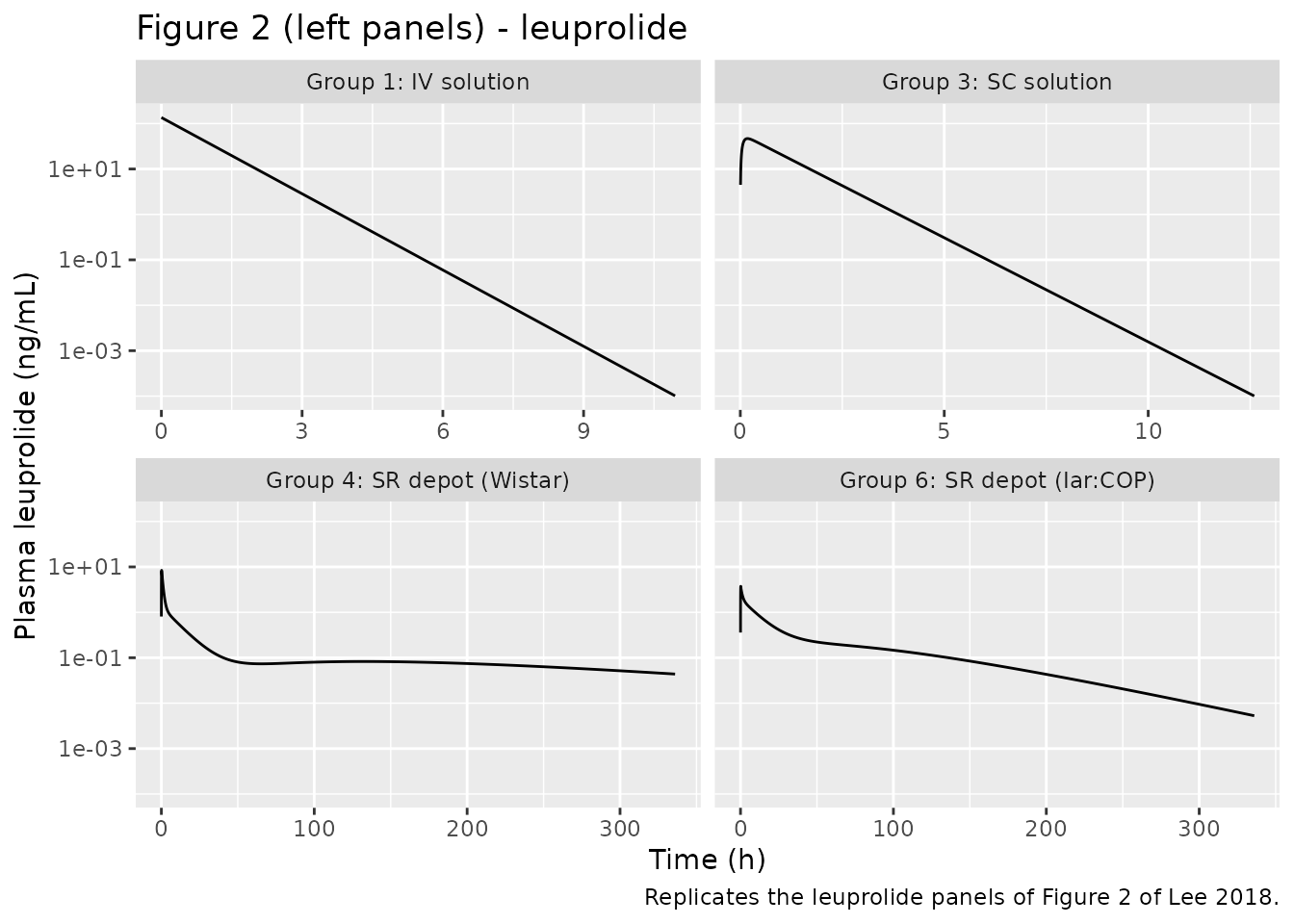
Note the x-axis unit. Figure 2’s leuprolide panels are labelled “Time
(day)”, but for the two solution groups they are in
hours: the drawn line falls five log10 units across
eight x-units, i.e. a slope of 1.44 per unit, which is the reported
elimination rate constant k = 1.42 1/h and not any per-day
quantity; and panel B’s peak sits at x ~ 0.18, which is the analytic
Tmax computed below. This is recorded as an erratum.
Figure 2, testosterone
# Replicates the right-hand testosterone panels of Figure 2 of Lee 2018.
sim |>
  ggplot(aes(day, TT)) +
  geom_line() +
  geom_hline(aes(yintercept = rbase_tt), linetype = "dashed", colour = "grey50") +
  facet_wrap(~group) +
  scale_y_log10() +
  labs(
    x = "Time (day)", y = "Plasma testosterone (ng/mL)",
    title = "Figure 2 (right panels) - testosterone",
    caption = paste(
      "Replicates the testosterone panels of Figure 2 of Lee 2018.",
      "Dashed line is the published baseline R0 (Equations 12 and 13)."
    )
  )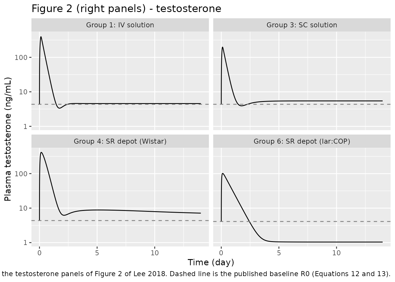
The shape is the paper’s: a sharp flare-up within the first hours, a nadir below baseline around day 1-2, and recovery to a plateau. The amplitude of the flare is not reproduced; see Errata item 2.
Figure 5, model schematic
Figure 5’s schematic is reproduced structurally by the compartment metadata:
purrr_free <- function(u) {
  cd <- u$compartmentData
  tibble::tibble(State = names(cd), Analyte = vapply(cd, `[[`, character(1), "analyte"))
}
purrr_free(uis[["Lee_2018_leuprolide_sr_rat"]]) |>
knitr::kable(caption = "States of the sustained-release model (Figure 5b of Lee 2018).")| State | Analyte |
|---|---|
| depot | leuprolide |
| depot2 | leuprolide |
| transit1 | leuprolide |
| transit2 | leuprolide |
| central | leuprolide |
| TT | testosterone |
| moderator1 | hypothalamo-pituitary-gonadal feedback signal |
Validation
Check 1 - release-section fractions and Equation (7)
The three release fractions are held on a 2-simplex by a stick-breaking logit pair rather than as three free parameters, so the first thing to prove is that the encoding returns Table 2 unchanged and that Equation (7) holds identically.
fracs <- sim |>
  dplyr::filter(model %in% c("Lee_2018_leuprolide_sr_rat", "Lee_2018_leuprolide_sr_cancer_rat")) |>
  dplyr::group_by(group) |>
  dplyr::summarise(NR = dplyr::first(frel), DR = dplyr::first(frel2), ER = dplyr::first(frel3), .groups = "drop") |>
  dplyr::mutate(sum = NR + DR + ER)
knitr::kable(fracs, digits = 10, caption = "Release fractions recovered from the stick-breaking encoding.")| group | NR | DR | ER | sum |
|---|---|---|---|---|
| Group 4: SR depot (Wistar) | 0.18 | 0.28 | 0.54 | 1 |
| Group 6: SR depot (Iar:COP) | 0.08 | 0.43 | 0.49 | 1 |
published_fracs <- tibble::tibble(NR = c(0.18, 0.08), DR = c(0.28, 0.43), ER = c(0.54, 0.49))
stopifnot(
  # Deterministic algebra, so an exact comparison is the right assertion.
  max(abs(fracs$NR - published_fracs$NR)) < 1e-12,
  max(abs(fracs$DR - published_fracs$DR)) < 1e-12,
  max(abs(fracs$ER - published_fracs$ER)) < 1e-12,
  max(abs(fracs$sum - 1)) < 1e-12
)
Check 2 - mass balance of the three-section depot
All of NR, DR and ER
eventually reach the central compartment and nothing is lost on the way,
so AUC(0-inf) * CL must equal the administered amount
exactly. This is a real test of the depot plumbing: a mis-wired transit
chain, a dropped f() fraction or a lag applied to the wrong
state all break it. Because the depot’s erosion chain has a mean transit
time of 2 / kt = 10.7 days for the Wistar group, a large
part of the dose is still unreleased at day 14, so the remaining amount
is added back explicitly.
state_cols <- c("depot", "depot2", "transit1", "transit2", "central")
mass <- lapply(model_names, function(nm) {
  r <- sims[[nm]]
  last_row <- r[nrow(r), , drop = FALSE]
  tibble::tibble(
    model = nm,
    auc_336 = sum(diff(r$time) * (head(r$Cc, -1) + tail(r$Cc, -1)) / 2),
    cl = r$cl[1],
    # Drug still in the depot / transit / central states at day 14 will all
    # eventually be cleared, so it contributes `amount / CL` to AUC(0-inf).
    remaining = sum(unlist(last_row[intersect(state_cols, names(last_row))]))
  )
}) |>
  dplyr::bind_rows() |>
  dplyr::left_join(spec, by = "model") |>
  dplyr::mutate(
    auc_inf = auc_336 + remaining / cl,
    recovered = auc_inf * cl,
    ratio = recovered / amt
  )

mass |>
  dplyr::select(group, `AUC 0-336 h` = auc_336, `AUC 0-inf` = auc_inf, `Recovered (ng)` = recovered, `Dose (ng)` = amt, Ratio = ratio) |>
knitr::kable(digits = c(0, 3, 3, 1, 1, 6), caption = "Mass balance: AUC(0-inf) x CL against the administered amount.")| group | AUC 0-336 h | AUC 0-inf | Recovered (ng) | Dose (ng) | Ratio |
|---|---|---|---|---|---|
| Group 1: IV solution | 105.503 | 105.503 | 26229.1 | 26228.4 | 1.000029 |
| Group 3: SC solution | 53.330 | 53.330 | 27436.0 | 27436.2 | 0.999993 |
| Group 4: SR depot (Wistar) | 45.548 | 53.330 | 27436.2 | 27436.2 | 1.000004 |
| Group 6: SR depot (Iar:COP) | 53.014 | 53.330 | 27436.3 | 27436.2 | 1.000006 |
Check 3 - analytic PK identities against Table 1
t1/2 is log(2) * Vd / CL and, for the
subcutaneous solution, Tmax = log(ka / kel) / (ka - kel).
Neither depends on the dose, so unlike the AUC comparison below these
are independent of the back-solved amount.
kel_iv <- 248.61 / 192.95
kel_sc <- 514.46 / 487.40
ka_sc <- 16.67

analytic <- tibble::tibble(
  Quantity = c("t1/2, IV solution (h)", "t1/2, SC solution (h)", "Tmax, SC solution (h)"),
  Model = c(log(2) / kel_iv, log(2) / kel_sc, log(ka_sc / kel_sc) / (ka_sc - kel_sc)),
  Published = c(0.52, 0.66, NA_real_),
  Source = c("Table 1, IV, row t 1/2", "Table 1, SC, row t 1/2", "not reported; Figure 2B peak sits at x ~ 0.18")
) |>
  dplyr::mutate(`% diff` = (Model - Published) / Published * 100)
knitr::kable(analytic, digits = 4, caption = "Analytic PK identities against Table 1.")| Quantity | Model | Published | Source | % diff |
|---|---|---|---|---|
| t1/2, IV solution (h) | 0.5380 | 0.52 | Table 1, IV, row t 1/2 | 3.4542 |
| t1/2, SC solution (h) | 0.6567 | 0.66 | Table 1, SC, row t 1/2 | -0.5018 |
| Tmax, SC solution (h) | 0.1767 | NA | not reported; Figure 2B peak sits at x ~ 0.18 | NA |
# Deterministic; 6% admits the internal inconsistency of Table 1 (its k, CL/Vd
# and t1/2 columns disagree by up to 10% because each is a mean of per-animal
# values), and still goes red on any transcription error in CL or Vd.
stopifnot(max(abs(analytic$`% diff`), na.rm = TRUE) < 6)
Table 1 reports k, CL and Vd
as separate per-animal means that are not mutually consistent
(CL / Vd = 1.288 1/h for the IV group against a reported
k of 1.42 1/h and a t1/2 of 0.52 h, i.e. 1.33
1/h). Equation (2) writes the elimination term as CL / Vd,
so that is what the model uses and k is left derived.
Check 4 - observed-Cmax comparison
Table 1’s Cmax values are the highest observed
samples, and the earliest sample was at 0.25 h. The like-for-like model
quantity is therefore the concentration at 0.25 h, not the peak of the
continuous curve (which for an IV bolus is the back-extrapolated
C0 = dose / Vd).
c025 <- sim |>
  dplyr::filter(model %in% model_names[1:2], abs(time - 0.25) < 1e-9) |>
  dplyr::select(group, Cc)
cmax_tab <- c025 |>
  dplyr::mutate(
    `Published Cmax` = c(97.10, 41.53),
    `% diff` = (Cc - `Published Cmax`) / `Published Cmax` * 100
  ) |>
  dplyr::rename("Model C at 0.25 h" = Cc)
knitr::kable(cmax_tab, digits = 3, caption = "Model concentration at the first sampling time against Table 1 Cmax.")| group | Model C at 0.25 h | Published Cmax | % diff |
|---|---|---|---|
| Group 1: IV solution | 98.499 | 97.10 | 1.441 |
| Group 3: SC solution | 45.227 | 41.53 | 8.901 |
Check 5 - PKNCA against Table 1
sim_nca <- sim |>
  dplyr::filter(model %in% model_names[1:2], time <= 12) |>
  dplyr::filter(!is.na(Cc)) |>
  dplyr::mutate(id = as.integer(factor(model))) |>
  dplyr::select(id, time, Cc, group)

# The time-zero row is already present from the solve (Cc = C0 for the IV bolus,
# 0 for the subcutaneous route), so the defensive row below is a no-op that
# distinct() discards; it is kept so the guarantee is explicit.
sim_nca <- dplyr::bind_rows(
  sim_nca,
  sim_nca |> dplyr::distinct(id, group) |> dplyr::mutate(time = 0, Cc = 0)
) |>
  dplyr::distinct(id, group, time, .keep_all = TRUE) |>
  dplyr::arrange(id, group, time)

conc_obj <- PKNCA::PKNCAconc(sim_nca, Cc ~ time | group + id)

dose_df <- sim_nca |>
  dplyr::distinct(id, group) |>
  dplyr::mutate(time = 0, amt = ifelse(id == 1L, dose_iv, dose_sc))
dose_obj <- PKNCA::PKNCAdose(dose_df, amt ~ time | group + id)

intervals <- data.frame(
  start = 0, end = Inf,
  cmax = TRUE, auclast = TRUE, aucinf.obs = TRUE, half.life = TRUE
)
nca_res <- PKNCA::pk.nca(PKNCA::PKNCAdata(conc_obj, dose_obj, intervals = intervals))
published <- tibble::tibble(
  group = levels(spec$group)[1:2],
  # Table 1 Cmax for the IV group is the highest observed sample (0.25 h), not
  # the back-extrapolated C0 that PKNCA reports here, so it is left out of the
  # comparison; Check 4 makes the like-for-like comparison instead.
  cmax = c(NA_real_, 41.53),
  auclast = c(103.44, 51.20),
  aucinf.obs = c(105.50, 53.33),
  half.life = c(0.52, 0.66)
)

cmp <- nlmixr2lib::ncaComparisonTable(
  simulated = nca_res,
  reference = published,
  by = "group",
  # half.life = TRUE also emits span.ratio / r.squared / lambda.z diagnostics;
  # restrict to the parameters the paper actually reports.
  params = c("cmax", "auclast", "aucinf.obs", "half.life"),
  units = c(cmax = "ng/mL", auclast = "h*ng/mL", aucinf.obs = "h*ng/mL", half.life = "h"),
  tolerance_pct = 20
)
knitr::kable(cmp, caption = "Simulated vs Table 1 NCA. * differs from reference by >20%.")| NCA parameter | group | Reference | Simulated | % diff |
|---|---|---|---|---|
| Cmax (ng/mL) | Group 1: IV solution | — | 136 | — |
| Cmax (ng/mL) | Group 3: SC solution | 41.5 | 46.7 | +12.5% |
| AUC0-∞ (obs) (h*ng/mL) | Group 1: IV solution | 106 | 105 | -0.0% |
| AUC0-∞ (obs) (h*ng/mL) | Group 3: SC solution | 53.3 | 53.3 | -0.0% |
| AUClast (h*ng/mL) | Group 1: IV solution | 103 | 105 | +2.0% |
| AUClast (h*ng/mL) | Group 3: SC solution | 51.2 | 53.3 | +4.2% |
| t½ (h) | Group 1: IV solution | 0.52 | 0.538 | +3.5% |
| t½ (h) | Group 3: SC solution | 0.66 | 0.657 | -0.5% |
attr(cmp, "footnote")
#> NULL
The two AUC rows are a transcription check, not an
independent gate. The administered amount was back-solved as
AUC0-inf x CL from this very table, so
AUC0-inf = dose / CL holds by construction; what the row
actually proves is that the model’s CL was transcribed
correctly and that the solver conserves mass. The half.life
and subcutaneous cmax rows are independent of the dose and
are the informative ones.
Check 6 - closed-form steady state of the feedback loop
Away from drug (ce -> 0), Equations (14) and (15)
have the joint fixed point
obtained by setting both derivatives to zero. Comparing that closed
form against the numerically integrated trajectory tests that the two
coupled ODEs were encoded as written - a sign error, a swapped rate
constant or a missing division by R all move the fixed
point.
ss <- sim |>
  dplyr::group_by(group) |>
  dplyr::summarise(
    closed_form = sqrt(dplyr::first(kin_tt) * dplyr::first(kin_moderator1) /
      (dplyr::first(kout_tt) * dplyr::first(kout_moderator1))),
    solved_14d = dplyr::last(TT),
    .groups = "drop"
  ) |>
  dplyr::mutate(ratio = solved_14d / closed_form)
knitr::kable(ss, digits = 4, caption = "Closed-form joint steady state against the trajectory at day 14.")| group | closed_form | solved_14d | ratio |
|---|---|---|---|
| Group 1: IV solution | 4.5705 | 4.5705 | 1.0000 |
| Group 3: SC solution | 5.4544 | 5.4544 | 1.0000 |
| Group 4: SR depot (Wistar) | 6.5192 | 7.1484 | 1.0965 |
| Group 6: SR depot (Iar:COP) | 1.0373 | 1.0373 | 1.0000 |
# Groups 1, 3 and 6 have essentially no drug left at day 14 and must sit on the
# fixed point exactly. Group 4's depot is still releasing (erosion mean transit
# time ~10.7 days), so its trajectory is legitimately still above the drug-free
# fixed point and is excluded.
stopifnot(max(abs(ss$ratio[c(1, 2, 4)] - 1)) < 1e-4)
The same closed form is what localises the Group 6 problem: it reproduces the Figure 2 plateaus of all three Wistar groups but not Group 6’s. See Errata item 3.
Check 7 - drug-free behaviour against the vehicle groups
Groups 2 and 5 received vehicle only and showed no change in testosterone over the whole experiment (“The dispersion solution did not induce any significant changes for the entire experimental period”, Results 2.3). Solving each model with no dose is the corresponding test.
vehicle <- lapply(model_names, function(nm) {
  as.data.frame(rxode2::rxSolve(uis[[nm]], rxode2::et(grid, cmt = "TT"), atol = 1e-12, rtol = 1e-10, useLinCmt = FALSE)) |>
    dplyr::mutate(model = nm)
}) |>
  dplyr::bind_rows() |>
  dplyr::left_join(spec, by = "model") |>
  dplyr::group_by(group) |>
  dplyr::summarise(
    `R0 (Eq 12/13)` = dplyr::first(rbase_tt),
    `kin / kout` = dplyr::first(kin_tt) / dplyr::first(kout_tt),
    `TT at day 14` = dplyr::last(TT),
    `% drift from R0` = (dplyr::last(TT) - dplyr::first(rbase_tt)) / dplyr::first(rbase_tt) * 100,
    .groups = "drop"
  )
knitr::kable(vehicle, digits = 3, caption = "Drug-free trajectory: published baseline against where the coupled system settles.")| group | R0 (Eq 12/13) | kin / kout | TT at day 14 | % drift from R0 |
|---|---|---|---|---|
| Group 1: IV solution | 4.353 | 4.250 | 4.571 | 4.997 |
| Group 3: SC solution | 4.353 | 4.250 | 5.454 | 25.301 |
| Group 4: SR depot (Wistar) | 4.353 | 4.250 | 6.519 | 49.763 |
| Group 6: SR depot (Iar:COP) | 4.094 | 5.833 | 1.037 | -74.664 |
The drug-free baseline is not flat for any group,
because the published R0, kin / kout and
sqrt(kin kf,on / (kout kf,off)) are three different numbers
in every column of Table 4. For the three Wistar groups the drift is
5-50% over 14 days and the settled level still brackets the observed
post-nadir plateau; for Group 6 the system falls fourfold. This is a
property of the published parameter set, not of the encoding - see
Errata items 3 and 4.
Documented deviations
The one aspect of the paper that this implementation does not reproduce is the amplitude of the testosterone flare. It is recorded here rather than tuned away, and is deliberately excluded from the assertions above.
flare <- sim |>
  dplyr::group_by(group) |>
  dplyr::summarise(
    `Model peak TT (ng/mL)` = max(TT),
    `at (h)` = time[which.max(TT)],
    .groups = "drop"
  ) |>
  dplyr::mutate(
    `Figure 2 fitted peak (read)` = c(65, 45, 110, 45),
    `Ratio` = `Model peak TT (ng/mL)` / `Figure 2 fitted peak (read)`
  )
knitr::kable(flare, digits = 2, caption = "KNOWN DEVIATION: flare amplitude. Not asserted; see Errata item 2.")| group | Model peak TT (ng/mL) | at (h) | Figure 2 fitted peak (read) | Ratio |
|---|---|---|---|---|
| Group 1: IV solution | 396.16 | 3.05 | 65 | 6.09 |
| Group 3: SC solution | 197.82 | 2.65 | 45 | 4.40 |
| Group 4: SR depot (Wistar) | 412.45 | 3.80 | 110 | 3.75 |
| Group 6: SR depot (Iar:COP) | 101.25 | 3.00 | 45 | 2.25 |
Assumptions and deviations (Errata)
-
Administered amount is back-solved, not reported. Body weight appears nowhere in the paper, so the 0.1 mg/kg dose could not be converted to an amount from the text. It was derived from the paper’s own
CL = Dose / AUC0-infdefinition, independently per route, giving 26,228 ng- and 27,436 ng (SC) and implied body weights of 262 g and 274 g. The
agreement between the two routes is the evidence that the derivation is
sound. A consequence: the
AUCrows of the PKNCA comparison are circular by construction and are labelled as such.
- and 27,436 ng (SC) and implied body weights of 262 g and 274 g. The
agreement between the two routes is the evidence that the derivation is
sound. A consequence: the
The flare-up amplitude is over-predicted by a factor of 2-6 for the three Wistar groups. Equations (14) and (16) with the Table 4 values give peak testosterone of 396 / 198 / 412 / 101 ng/mL for Groups 1 / 3 / 4 / 6, and the maximum prediction at an actual sampling time is 412 ng/mL. Figure 3D, the paper’s own weighted-residual plot, has predicted testosterone on its x-axis and it tops out at about 95 ng/mL; the fitted curves in Figure 2 peak at roughly 65 / 45 / 110 / 45 ng/mL. The one free quantity is the unstated initial condition of the feedback pool,
F(0), which the paper never gives. It cannot explain the pattern: the peak is very nearly proportional toF(0)while the nadir and the plateau are completely independent of it, so matching each group in turn would needF(0)= 0.16 / 0.23 / 0.27 / 0.44, not one value.F(0) = 1is used because it is the value at which Equation (14) collapses exactly onto the paper’s own baseline model, Equation (11), which is how the paper describes the drug-effect model being constructed. Nothing was tuned. Everything downstream of the flare - nadir depth, nadir timing and recovered plateau - does reproduce for the Wistar groups.The Group 6 (Iar:COP) feedback constants do not reproduce the paper’s own Figure 2D. The joint fixed point
sqrt(kin kf,on / (kout kf,off))gives 4.57 / 5.45 / 6.52 ng/mL for the three Wistar groups, matching the plateaus drawn in Figure 2A-C (about 4.5-5, 5.5 and 7). For Group 6 the same closed form gives 1.04 ng/mL against a plateau of about 4.2 in Figure 2D and an observed 3-14 day mean of 4.39 ng/mL reported in Results 2.3. Group 6 is also the only column of Table 4 whosekf,onis smaller than itskf,off(by a factor of 5.4, where the other three havekf,onlarger by 5-10x) and the only one whosekf,onstandard error (0.14) exceeds its point estimate (0.083). The published values are transcribed unchanged and the inconsistency is flagged in that model file’sdescription.R0is not the steady state of the model it initialises. Equation (11) is at rest whenR = kin / kout, which is 4.25 for Wistar against theR0 = 4.353of Equation (12) - consistent within 2.4% - but 5.83 for Iar:COP against theR0 = 4.094of Equation (13), a 42% disagreement. The full coupled system settles at a third value again. All three published numbers are kept as printed; the drug-free drift this produces is quantified in Check 7.F(0) = 1is an assumption, as above. The alternative of starting the pool at its own quasi-steady statekf,on / (kf,off R0)shifts the flare peak by about 13% for Group 1 and leaves the nadir and plateau unchanged.No between-animal variability and no residual error model are reported. Every
+/-in Tables 1-4 is the standard error of a parameter estimate across n = 5 animals, not a variance component: Methods 4.7 fits each group’s mean profile deterministically in Berkeley Madonna.propSdandpropSd_TTare thereforefixed(0)rather than invented, and the models carry noetaterms.Figure 2’s leuprolide x-axis is mislabelled for the solution groups. It reads “Time (day)” but is in hours - the fitted line’s slope is 1.44 per x-unit, which is the reported
k= 1.42 1/h, and panel B’s peak at x ~ 0.18 is the analyticTmaxof 0.177 h. The depot panels (C and D), which run to 14 days, are genuinely in days.Table 3’s AUEC values are not reproduced and no attempt is made to. They are computed from observed data by subtracting a baseline AUEC and splitting the remainder into positive and negative segments (Discussion, Methods 4.6), but the segmentation convention and the units are not specified. The paper’s own fitted curves recover above baseline after the nadir, so the model’s negative area is roughly fifty times smaller than the published figures; a numeric comparison would measure the undefined convention, not the model.
kf,onunits. Table 4 heads both thekf,onandkf,offrows “h - 1”. That is right forkf,off, but Equation (15) divideskf,onby a concentration, sokf,onmust carry ng/mL/h fordF/dtto be a pure 1/h rate. Thelabel()states the units the equation requires and records what the table prints.Disposition is shared across groups, as the paper specifies. The two depot models do not re-estimate
ka,CL/ForVd/F; Methods 4.7 builds the depot model “based on the PK parameters such as ka, CL, and Vd in solution-administered groups”, so those three are carried from Group 3 unchanged, including into the Iar:COP model. The paper notes that PK did not differ significantly between strains whileEmaxandEC50did.Naming. The paper’s
kdandktare encoded as the canonicallka2andlktr: Results 2.4 states that both “are rate constants that include both the release process in the biological systems and the absorption process of the released drug”, i.e. apparent first-order input rate constants, which is exactly what those canonicals denote. The three release fractionsNR/DR/ERare held by a stick-breakinglogitfrel/logitfrel2pair so that Equation (7) holds identically; Check 1 proves the printed values are recovered. The feedback pool is the canonicalmoderator1compartment withkin_moderator1/kout_moderator1rate constants, keeping it clear of the testosterone pool’skin_tt/kout_tt.