Atezolizumab in pediatric and young adult patients (Shemesh 2019)
Source:vignettes/articles/Shemesh_2019_atezolizumab.Rmd
Shemesh_2019_atezolizumab.RmdModel
Shemesh et al. (2019) refitted the adult two-compartment intravenous atezolizumab population PK model (Stroh et al. 2017) to 431 serum concentrations from 87 pediatric and young adult patients in the phase I/II iMATRIX-atezolizumab study, keeping the adult structure and re-estimating every parameter. Patients < 18 years received 15 mg/kg q3w (maximum 1200 mg); patients >= 18 years received 1200 mg q3w.
mod <- rxode2::rxode(readModelDb("Shemesh_2019_atezolizumab"))
#> ℹ parameter labels from comments will be replaced by 'label()'
mod$description
#> [1] "Two-compartment population PK model with intravenous infusion input for atezolizumab (anti-PD-L1 IgG1) in pediatric and young adult patients (7 months to 29 years, 8.7-154 kg) with relapsed or refractory solid tumors or lymphoma from the iMATRIX-atezolizumab phase I/II study (Shemesh 2019, n = 87, 431 serum concentrations). The adult atezolizumab popPK structure was refitted to the pediatric data with every parameter re-estimated: power effects of body weight and albumin on CL and V1, of baseline tumor burden on CL, and a multiplicative factor for treatment-emergent ADA on CL. Sex effects were not evaluated and V2 and Q carry no covariates."
Population
str(mod$population)
#> List of 15
#>  $ species         : chr "human"
#>  $ n_subjects      : num 87
#>  $ n_studies       : num 1
#>  $ n_observations  : num 431
#>  $ age_range       : chr "7 months to 29 years"
#>  $ age_median      : chr "12 years (69 patients < 18 years); 22 years (18 young adults)"
#>  $ weight_range    : chr "8.7-154 kg"
#>  $ weight_median   : chr "38.9 kg (< 18 years); 61.0 kg (>= 18 years)"
#>  $ sex_female_pct  : num 46
#>  $ disease_state   : chr "Relapsed or refractory pediatric solid tumors (Ewing sarcoma, neuroblastoma, osteosarcoma, rhabdomyosarcoma, no"| __truncated__
#>  $ dose_range      : chr "15 mg/kg IV q3w (maximum 1200 mg) for patients < 18 years; 1200 mg IV q3w flat for patients >= 18 years; 60-min"| __truncated__
#>  $ age_groups      : chr "2 infants < 2 y, 29 children 2 to < 12 y, 38 adolescents 12 to < 18 y, 18 young adults >= 18 y"
#>  $ ada_positive_pct: num 13
#>  $ regions         : chr "Multinational (iMATRIX-atezolizumab, NCT02541604)"
#>  $ notes           : chr "Shemesh 2019 Table 1 (baseline demographics by age group); 40 of 87 female."
Baseline characteristics by age group (Shemesh 2019 Table 1): 2 infants < 2 years (median 9.1 kg), 29 children 2 to < 12 years (22.5 kg), 38 adolescents 12 to < 18 years (51.1 kg) and 18 young adults >= 18 years (61.0 kg). Median albumin was 33-41 g/L and median tumor burden 55-120 mm across groups; 13% of patients were treatment-emergent ADA-positive.
Source trace
tibble::tribble(
  ~Quantity, ~Value, ~`Source location`,
  "CL (L/day)", "0.217", "Table 2",
  "V1 (L)", "3.01", "Table 2",
  "V2 (L)", "1.36", "Table 2",
  "Q (L/day)", "0.183", "Table 2",
  "WT exponent on CL", "0.795", "Table 2",
  "ALB exponent on CL", "-1.18", "Table 2",
  "TUMSZ exponent on CL", "0.122", "Table 2",
  "ADA factor on CL (theta^ADA)", "1.23", "Table 2; Methods 'PopPK model'; Discussion '23% increase'",
  "WT exponent on V1", "0.766", "Table 2",
  "ALB exponent on V1", "-0.566", "Table 2",
  "Sex on V1 / V2", "not evaluated", "Table 2 (NE)",
  "BSV CL / V1 / V2 (variance)", "0.0458 / 0.0140 / 0.311", "Table 2",
  "Correlation CL-V1", "0.510 (covariance 0.012914)", "Table 2",
  "Proportional residual variance", "0.051 (SD 0.2258)", "Table 2",
  "Additive residual variance", "68.9 (SD 8.301 ug/mL)", "Table 2",
  "Reference WT / ALB / TUMSZ", "77 kg / 40 g/L / 63 mm", "Methods adult CL and V1 equations",
  "Two-compartment IV infusion structure", "-", "Methods 'PopPK model'; Results",
  "Dosing and infusion durations", "15 mg/kg (max 1200) or 1200 mg q3w; 60 min then 30 min", "Methods 'Study design'"
) |>
knitr::kable()| Quantity | Value | Source location |
|---|---|---|
| CL (L/day) | 0.217 | Table 2 |
| V1 (L) | 3.01 | Table 2 |
| V2 (L) | 1.36 | Table 2 |
| Q (L/day) | 0.183 | Table 2 |
| WT exponent on CL | 0.795 | Table 2 |
| ALB exponent on CL | -1.18 | Table 2 |
| TUMSZ exponent on CL | 0.122 | Table 2 |
| ADA factor on CL (theta^ADA) | 1.23 | Table 2; Methods ‘PopPK model’; Discussion ‘23% increase’ |
| WT exponent on V1 | 0.766 | Table 2 |
| ALB exponent on V1 | -0.566 | Table 2 |
| Sex on V1 / V2 | not evaluated | Table 2 (NE) |
| BSV CL / V1 / V2 (variance) | 0.0458 / 0.0140 / 0.311 | Table 2 |
| Correlation CL-V1 | 0.510 (covariance 0.012914) | Table 2 |
| Proportional residual variance | 0.051 (SD 0.2258) | Table 2 |
| Additive residual variance | 68.9 (SD 8.301 ug/mL) | Table 2 |
| Reference WT / ALB / TUMSZ | 77 kg / 40 g/L / 63 mm | Methods adult CL and V1 equations |
| Two-compartment IV infusion structure | - | Methods ‘PopPK model’; Results |
| Dosing and infusion durations | 15 mg/kg (max 1200) or 1200 mg q3w; 60 min then 30 min | Methods ‘Study design’ |
Virtual cohort
Covariates are drawn per age group around the Table 1 medians and truncated to the Table 1 ranges (log-normal for weight and tumor burden, normal for albumin); ADA status is Bernoulli at the observed group rate.
set.seed(2019)
rxode2::rxSetSeed(2019)

groups <- tibble::tribble(
  ~agegrp, ~n, ~wt_med, ~wt_min, ~wt_max, ~alb_med, ~alb_min, ~alb_max, ~tum_med, ~tum_min, ~tum_max, ~ada,
  "< 2 y", 20, 9.1, 8.7, 9.5, 33, 30, 35, 59, 35, 83, 0,
  "2 to < 12 y", 150, 22.5, 12.0, 74.4, 41, 23, 46, 55, 15, 301, 0.17,
  "12 to < 18 y", 150, 51.1, 28.2, 105, 41, 29, 49, 78, 11, 208, 0.11,
  ">= 18 y", 150, 61.0, 46.2, 154, 39, 27, 47, 120, 10, 258, 0.11
)

rtrunc_lnorm <- function(n, med, lo, hi) {
  x <- exp(rnorm(n, log(med), (log(hi) - log(lo)) / 4))
  pmin(pmax(x, lo), hi)
}
rtrunc_norm <- function(n, med, lo, hi) {
  pmin(pmax(rnorm(n, med, (hi - lo) / 4), lo), hi)
}

cohort <- groups |>
  rowwise() |>
  reframe(
    agegrp = agegrp,
    WT = rtrunc_lnorm(n, wt_med, wt_min, wt_max),
    ALB = rtrunc_norm(n, alb_med, alb_min, alb_max),
    TUMSZ = rtrunc_lnorm(n, tum_med, tum_min, tum_max),
    ADA_POS = rbinom(n, 1, ada)
  ) |>
  mutate(
    id = row_number(),
    agegrp = factor(agegrp, levels = groups$agegrp),
    regimen = ifelse(agegrp == ">= 18 y", "1200 mg flat", "15 mg/kg"),
    dose = ifelse(regimen == "1200 mg flat", 1200, pmin(15 * WT, 1200)),
    wtband = case_when(
      regimen == "15 mg/kg" & WT < 30 ~ "< 18 y: < 30 kg",
      regimen == "15 mg/kg" & WT < 45 ~ "< 18 y: 30 to < 45 kg",
      regimen == "15 mg/kg" ~ "< 18 y: >= 45 kg",
      WT < 57 ~ ">= 18 y: < 57 kg",
      WT < 65 ~ ">= 18 y: 57 to < 65 kg",
      TRUE ~ ">= 18 y: >= 65 kg"
    )
  )

cohort |>
  group_by(agegrp) |>
  summarise(n = n(), WT = median(WT), ALB = median(ALB), TUMSZ = median(TUMSZ),
            `ADA+ (%)` = 100 * mean(ADA_POS)) |>
knitr::kable(digits = 1)| agegrp | n | WT | ALB | TUMSZ | ADA+ (%) |
|---|---|---|---|---|---|
| < 2 y | 20 | 9.0 | 33.0 | 61.0 | 0.0 |
| 2 to < 12 y | 150 | 21.0 | 40.6 | 59.8 | 20.7 |
| 12 to < 18 y | 150 | 48.3 | 40.6 | 88.3 | 16.0 |
| >= 18 y | 150 | 59.3 | 38.1 | 118.8 | 12.0 |
Event table
Ten q3w cycles; 60-min infusion in cycle 1 and 30-min infusions afterwards (Shemesh 2019 Methods). Cycle 1 and cycle 10 (steady state, as in the paper) are sampled densely; the cycle trough is read at day 20.99 of the cycle, the last sampling time the paper used.
tau <- 21
dose_times <- tau * (0:9)
ss_start <- dose_times[10]
grid1 <- sort(unique(c(0, seq(0.01, 3, by = 0.05), seq(3.5, 20.5, by = 0.5), 20.99)))
obs_times <- c(grid1, ss_start + grid1)

doses <- cohort |>
  select(id, dose) |>
  tidyr::crossing(time = dose_times) |>
  mutate(
    dur = ifelse(time == 0, 1 / 24, 0.5 / 24),
    amt = dose, rate = amt / dur, evid = 1, cmt = "central"
  ) |>
  select(id, time, amt, rate, evid, cmt)

obs <- cohort |>
  select(id) |>
  tidyr::crossing(time = obs_times) |>
  mutate(amt = 0, rate = 0, evid = 0, cmt = "central")

events <- bind_rows(doses, obs) |>
  left_join(select(cohort, id, WT, ALB, TUMSZ, ADA_POS), by = "id") |>
  arrange(id, time, desc(evid))
Simulation
sim <- rxode2::rxSolve(mod, events, returnType = "data.frame",
                       keep = c("WT", "ALB", "TUMSZ", "ADA_POS")) |>
  left_join(select(cohort, id, agegrp, regimen, wtband), by = "id")
sim |>
  mutate(cycle = ifelse(time < ss_start, "Cycle 1", "Cycle 10"),
         tcyc = ifelse(time < ss_start, time, time - ss_start)) |>
  group_by(agegrp, cycle, tcyc) |>
  summarise(med = median(Cc), lo = quantile(Cc, 0.05), hi = quantile(Cc, 0.95),
            .groups = "drop") |>
  # the pre-dose zero of cycle 1 cannot be drawn on a log axis
  filter(lo > 0) |>
  mutate(cycle = factor(cycle, levels = c("Cycle 1", "Cycle 10"))) |>
  ggplot(aes(tcyc, med, colour = agegrp, fill = agegrp)) +
  geom_ribbon(aes(ymin = lo, ymax = hi), alpha = 0.15, colour = NA) +
  geom_line() +
  geom_hline(yintercept = 6, linetype = "dotted") +
  facet_wrap(~cycle) +
  scale_y_log10() +
  labs(x = "Time after dose in cycle (day)", y = "Atezolizumab (ug/mL)",
       colour = "Age group", fill = "Age group")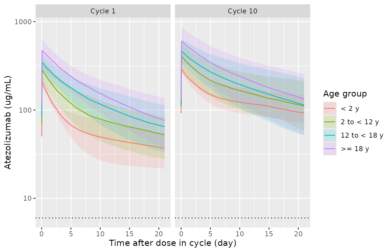
Simulated cycle 1 and cycle 10 profiles (median and 5th-95th percentiles) by age group. The dotted line is the 6 ug/mL target trough (Shemesh 2019 Fig. 3).
Cycle 1 trough by age group
Shemesh 2019 Results report geometric-mean cycle 1 Cmin of 55.9 ug/mL in children 2 to < 12 years and 62.4 ug/mL in adolescents 12 to < 18 years.
geo_mean <- function(x) exp(mean(log(x)))

cmin_age <- sim |>
  filter(abs(time - 20.99) < 1e-6) |>
  group_by(agegrp) |>
  summarise(sim_gm = geo_mean(Cc), .groups = "drop") |>
  inner_join(tibble::tibble(agegrp = c("2 to < 12 y", "12 to < 18 y"),
                            published = c(55.9, 62.4)), by = "agegrp") |>
  mutate(pct_diff = 100 * (sim_gm - published) / published)
cmin_age |>
  dplyr::rename("Age group" = agegrp, "Simulated GM Cmin (ug/mL)" = sim_gm,
                "Published GM Cmin (ug/mL)" = published, "% diff" = pct_diff) |>
knitr::kable(digits = 1)| Age group | Simulated GM Cmin (ug/mL) | Published GM Cmin (ug/mL) | % diff |
|---|---|---|---|
| 2 to < 12 y | 49.8 | 55.9 | -10.9 |
| 12 to < 18 y | 62.7 | 62.4 | 0.5 |
PKNCA validation
Cycle 1 (days 0-20.99) and cycle 10 (days 189-209.99) intervals. The PKNCA grouping is the Table 3 dose regimen / weight band.
conc_df <- sim |>
  filter(!is.na(Cc)) |>
  select(id, time, Cc, wtband)
dose_df <- doses |>
  left_join(select(cohort, id, wtband), by = "id") |>
  select(id, time, amt, wtband)

conc_obj <- PKNCA::PKNCAconc(conc_df, Cc ~ time | wtband + id)
dose_obj <- PKNCA::PKNCAdose(dose_df, amt ~ time | wtband + id)
intervals <- data.frame(
  start = c(0, ss_start), end = c(20.99, ss_start + 20.99),
  cmax = TRUE, cmin = TRUE, auclast = TRUE
)
nca <- PKNCA::pk.nca(PKNCA::PKNCAdata(conc_obj, dose_obj, intervals = intervals))

nca_res <- as.data.frame(nca) |>
  filter(PPTESTCD %in% c("cmax", "cmin", "auclast")) |>
  mutate(cycle = ifelse(start == 0, "Cycle 1", "Steady state"))
# Cycle 1 minimum over [0, 20.99] is the pre-dose zero; use the end-of-cycle
# trough instead, which is how the paper defines cycle 1 Cmin.
cmin_c1 <- sim |>
  filter(abs(time - 20.99) < 1e-6) |>
  transmute(wtband, id, cycle = "Cycle 1", PPTESTCD = "cmin", PPORRES = Cc)
sim_long <- nca_res |>
  filter(!(cycle == "Cycle 1" & PPTESTCD == "cmin")) |>
  select(wtband, id, cycle, PPTESTCD, PPORRES) |>
  bind_rows(cmin_c1)
Comparison against Shemesh 2019 Table 3
Table 3 reports medians of the individual post-hoc exposures by dose regimen and weight band; the simulated values are medians over the virtual cohort.
bands <- c("< 18 y: < 30 kg", "< 18 y: 30 to < 45 kg", "< 18 y: >= 45 kg",
           ">= 18 y: < 57 kg", ">= 18 y: 57 to < 65 kg", ">= 18 y: >= 65 kg")
published <- bind_rows(
  tibble::tibble(wtband = bands, cycle = "Cycle 1",
                 cmax = c(270, 330, 349, 492, 486, 326),
                 cmin = c(55.6, 65.0, 65.5, 97.3, 98.8, 57.6),
                 auclast = c(2085, 2757, 2988, 4268, 4330, 2733)),
  tibble::tibble(wtband = bands, cycle = "Steady state",
                 cmax = c(400, 463, 460, 664, 651, 404),
                 cmin = c(120, 125, 112, 171, 164, 88.1),
                 auclast = c(4045, 4781, 4510, 6692, 6574, 3861))
) |>
  pivot_longer(c(cmax, cmin, auclast), names_to = "PPTESTCD", values_to = "PPORRES")

cmp <- nlmixr2lib::ncaComparisonTable(
  simulated = sim_long,
  reference = published,
  by = c("wtband", "cycle"),
  units = c(cmax = "ug/mL", cmin = "ug/mL", auclast = "ug*day/mL"),
  tolerance_pct = 20
)
cmp |>
  dplyr::rename("Regimen / weight band" = wtband, "Cycle" = cycle) |>
knitr::kable(caption = "Simulated medians vs Shemesh 2019 Table 3. * differs by more than 20%.")| NCA parameter | Regimen / weight band | Cycle | Reference | Simulated | % diff |
|---|---|---|---|---|---|
| Cmax (ug/mL) | < 18 y: < 30 kg | Cycle 1 | 270 | 267 | -1.2% |
| Cmax (ug/mL) | < 18 y: < 30 kg | Steady state | 400 | 380 | -5.1% |
| Cmax (ug/mL) | < 18 y: 30 to < 45 kg | Cycle 1 | 330 | 319 | -3.4% |
| Cmax (ug/mL) | < 18 y: 30 to < 45 kg | Steady state | 463 | 448 | -3.3% |
| Cmax (ug/mL) | < 18 y: >= 45 kg | Cycle 1 | 349 | 359 | +3.0% |
| Cmax (ug/mL) | < 18 y: >= 45 kg | Steady state | 460 | 479 | +4.1% |
| Cmax (ug/mL) | >= 18 y: < 57 kg | Cycle 1 | 492 | 548 | +11.3% |
| Cmax (ug/mL) | >= 18 y: < 57 kg | Steady state | 664 | 718 | +8.1% |
| Cmax (ug/mL) | >= 18 y: 57 to < 65 kg | Cycle 1 | 486 | 482 | -0.8% |
| Cmax (ug/mL) | >= 18 y: 57 to < 65 kg | Steady state | 651 | 624 | -4.2% |
| Cmax (ug/mL) | >= 18 y: >= 65 kg | Cycle 1 | 326 | 363 | +11.4% |
| Cmax (ug/mL) | >= 18 y: >= 65 kg | Steady state | 404 | 463 | +14.5% |
| Cmin (ug/mL) | < 18 y: < 30 kg | Cycle 1 | 55.6 | 47.6 | -14.4% |
| Cmin (ug/mL) | < 18 y: < 30 kg | Steady state | 120 | 107 | -10.9% |
| Cmin (ug/mL) | < 18 y: 30 to < 45 kg | Cycle 1 | 65 | 59.1 | -9.1% |
| Cmin (ug/mL) | < 18 y: 30 to < 45 kg | Steady state | 125 | 112 | -10.1% |
| Cmin (ug/mL) | < 18 y: >= 45 kg | Cycle 1 | 65.5 | 66.5 | +1.5% |
| Cmin (ug/mL) | < 18 y: >= 45 kg | Steady state | 112 | 115 | +2.8% |
| Cmin (ug/mL) | >= 18 y: < 57 kg | Cycle 1 | 97.3 | 95.4 | -2.0% |
| Cmin (ug/mL) | >= 18 y: < 57 kg | Steady state | 171 | 164 | -4.1% |
| Cmin (ug/mL) | >= 18 y: 57 to < 65 kg | Cycle 1 | 98.8 | 69.7 | -29.5%* |
| Cmin (ug/mL) | >= 18 y: 57 to < 65 kg | Steady state | 164 | 141 | -14.0% |
| Cmin (ug/mL) | >= 18 y: >= 65 kg | Cycle 1 | 57.6 | 64.7 | +12.4% |
| Cmin (ug/mL) | >= 18 y: >= 65 kg | Steady state | 88.1 | 99.5 | +13.0% |
| AUClast (ug*day/mL) | < 18 y: < 30 kg | Cycle 1 | 2080 | 1810 | -13.0% |
| AUClast (ug*day/mL) | < 18 y: < 30 kg | Steady state | 4040 | 3620 | -10.6% |
| AUClast (ug*day/mL) | < 18 y: 30 to < 45 kg | Cycle 1 | 2760 | 2570 | -6.8% |
| AUClast (ug*day/mL) | < 18 y: 30 to < 45 kg | Steady state | 4780 | 4220 | -11.8% |
| AUClast (ug*day/mL) | < 18 y: >= 45 kg | Cycle 1 | 2990 | 3050 | +2.2% |
| AUClast (ug*day/mL) | < 18 y: >= 45 kg | Steady state | 4510 | 4730 | +4.8% |
| AUClast (ug*day/mL) | >= 18 y: < 57 kg | Cycle 1 | 4270 | 4390 | +3.0% |
| AUClast (ug*day/mL) | >= 18 y: < 57 kg | Steady state | 6690 | 6720 | +0.3% |
| AUClast (ug*day/mL) | >= 18 y: 57 to < 65 kg | Cycle 1 | 4330 | 4030 | -7.0% |
| AUClast (ug*day/mL) | >= 18 y: 57 to < 65 kg | Steady state | 6570 | 5940 | -9.7% |
| AUClast (ug*day/mL) | >= 18 y: >= 65 kg | Cycle 1 | 2730 | 3180 | +16.5% |
| AUClast (ug*day/mL) | >= 18 y: >= 65 kg | Steady state | 3860 | 4480 | +15.9% |
pct <- sim_long |>
  group_by(wtband, cycle, PPTESTCD) |>
  summarise(sim = median(PPORRES), .groups = "drop") |>
  inner_join(published, by = c("wtband", "cycle", "PPTESTCD")) |>
  mutate(pct_diff = 100 * (sim - PPORRES) / PPORRES)
stopifnot(
  abs(median(pct$pct_diff)) < 10,
  quantile(abs(pct$pct_diff), 0.75) < 25
)
The pediatric weight bands (n = 21-25 patients each in the study) agree within about 15% for every metric. The largest differences are in the young-adult bands, each of which holds only 6 study patients, so their Table 3 medians are driven by individual covariate values that a Table 1-based virtual cohort does not reproduce (for example the cycle 1 Cmin of the 57 to < 65 kg band).
Typical-value half-life
Shemesh 2019 Results: terminal half-life of ~2-3 weeks in pediatric patients and young adults. The terminal half-life of the typical patient in each age group follows directly from the micro-constants.
thalf <- groups |>
  transmute(
    agegrp,
    cl = 0.217 * (wt_med / 77)^0.795 * (alb_med / 40)^-1.18 * (tum_med / 63)^0.122,
    vc = 3.01 * (wt_med / 77)^0.766 * (alb_med / 40)^-0.566,
    vp = 1.36, q = 0.183
  ) |>
  mutate(
    kel = cl / vc, k12 = q / vc, k21 = q / vp,
    beta = 0.5 * ((kel + k12 + k21) - sqrt((kel + k12 + k21)^2 - 4 * kel * k21)),
    t_half_day = log(2) / beta
  )
knitr::kable(select(thalf, agegrp, cl, vc, t_half_day), digits = 3)| agegrp | cl | vc | t_half_day |
|---|---|---|---|
| < 2 y | 0.049 | 0.654 | 31.894 |
| 2 to < 12 y | 0.078 | 1.157 | 25.447 |
| 12 to < 18 y | 0.156 | 2.168 | 18.068 |
| >= 18 y | 0.201 | 2.554 | 15.775 |
# Deterministic: typical adolescents and young adults fall in the 2-3 week band.
stopifnot(all(thalf$t_half_day[thalf$agegrp %in% c("12 to < 18 y", ">= 18 y")] > 14 &
  thalf$t_half_day[thalf$agegrp %in% c("12 to < 18 y", ">= 18 y")] < 21))
The typical child (22.5 kg) and infant (9.1 kg) have longer terminal half-lives (about 3.6 and 4.6 weeks), because V2 and Q are not scaled by body weight in the pediatric model while CL and V1 are. The paper’s “~2-3 weeks” statement summarizes individual post-hoc estimates across all patients, most of whom are adolescents, and the authors note that infant results “have limited interpretation”.
Assumptions and deviations
- Reference covariate values. The paper prints the normalization references (77 kg, 40 g/L, 63 mm) only for the adult equations; the pediatric model “utilized the same structure”, so the same references are used here.
-
ADA effect form. Per the Methods, the pediatric ADA
effect is parameterized
theta^ADA(1.23), unlike the adult(1 + theta)form. - Residual error. Table 2 reports variances; the model carries their square roots. The additive component is taken to be on the ug/mL scale, consistent with the adult model and the reported concentrations.
- IIV. Exponential (log-normal) between-subject variability assumed on CL, V1 and V2 as in the adult model; only the CL-V1 correlation was estimated.
- Sex was not evaluated (NE) in the pediatric model and is omitted; the adult-model sex effects are not carried over.
-
Adult model column of Table 2. The adult comparator
(Stroh 2017) is not extracted here; its disposition parameters ship as
the fixed IV layer of
Chan_2025_atezolizumab. - Virtual cohort. Covariate distributions are approximated from Table 1 medians and ranges; the 2 infants of the study are represented by 20 simulated infants. ADA status is treated as time-constant.
- Table 3 comparison. Table 3 is based on the study’s individual post-hoc parameters, so the comparison with a virtual cohort is approximate and is asserted on the median and interquartile envelope rather than every cell.