Model and source
- Citation: Zhu K, Ding X, Xue L, Liu L, Wang Y, Li Y, Xi Q, Pang X, Chen W, Miao L. Optimising infliximab induction dosing to achieve clinical remission in Chinese patients with Crohn’s disease. Front Pharmacol. 2024;15:1430120. doi:10.3389/fphar.2024.1430120
- Description: One-compartment IV population PK model of infliximab in Chinese patients with Crohn’s disease, with fat-free mass on clearance and volume and serum albumin and antibody-to-infliximab titre on clearance (Zhu 2024)
- Article: https://doi.org/10.3389/fphar.2024.1430120 (open access)
- Supplement: Supplementary Material (DOCX) with the final parameter table (Table S5), the covariate bootstrap (Table S3) and the backward-elimination table (Table S4).
Zhu et al. related early infliximab trough levels and antibodies to infliximab (ATI) to clinical remission at week 14 in Chinese patients with Crohn’s disease, then used a population PK model fitted to 526 samples from 140 patients to simulate the probability of reaching the week-2 trough target of 20.08 ug/mL across induction doses, body weights and albumin levels. The PK model is one-compartment with first-order elimination after IV infusion:
with = 1 for ATI absent or titre 1:20, 1.17 for titre 1:60 and 1.38 for titre >= 1:180.
Population
The model was developed in 140 patients with Crohn’s disease treated at the First Affiliated Hospital of Soochow University, China, between October 2020 and December 2022 (Table 1): 106 men and 34 women, median age 34 years (range 15-58), mean weight 59.9 kg (SD 10.8, range 39-80), median baseline albumin 38.3 g/L (IQR 34.4-43.1). Induction doses were 200 mg (19 patients), 300 mg (105) or 400 mg (16) at weeks 0, 2 and 6, then every 8 weeks. ATI were detected in 234 of 526 samples (1:20 in 96, 1:60 in 86, >= 1:180 in 52), and 66 samples (12.6%) were below the 0.50 ug/mL quantification limit, almost all from ATI-positive patients.
The same information is available programmatically via
readModelDb("Zhu_2024_infliximab")$population.
Source trace
| Equation / parameter | Value | Source location |
|---|---|---|
| One-compartment, first-order elimination | n/a | Results, “Modelling” |
lcl (CL, reference patient) |
0.45 L/day | Table S5; Eq. 4 |
lvc (V, reference patient) |
9.65 L | Table S5; Eq. 3 |
e_ffm_cl (FFM exponent on CL, reference 56.1 kg) |
0.75 (fixed) | Eq. 4 |
e_ffm_vc (FFM exponent on V, reference 56.1 kg) |
1 (fixed) | Eq. 3 |
e_alb_cl (albumin exponent on CL, reference 40
g/L) |
-0.48 | Table S5; Eq. 4 |
e_ada60_cl (CL factor, ATI titre 1:60) |
1.17 | Table S5; Eq. 4 |
e_ada180_cl (CL factor, ATI titre >= 1:180) |
1.38 | Table S5; Eq. 4 |
etalcl (IIV on CL) |
25.1% CV, variance 0.0611 | Table S5 |
propSd |
26.6% | Table S5 |
addSd |
0.15 ug/mL | Table S5 |
| FFM from weight, height and sex | Janmahasatian 2005 | Methods, “popPK modelling” |
| Exponential IIV; combined proportional + additive error | n/a | Methods, “popPK modelling” |
Fat-free mass
The model takes fat-free mass directly. The helper below applies the Janmahasatian formula the authors cite.
Typical-value profiles
The reference patient (FFM 56.1 kg, albumin 40 g/L) receives 300 mg
at weeks 0, 2 and 6 and every 8 weeks thereafter, without ATI and at
each ATI titre class. With CL = 0.45 L/day and V = 9.65 L, the
elimination half-life is log(2) * 9.65 / 0.45 = 14.9
days.
mod <- readModelDb("Zhu_2024_infliximab")
mod_typ <- rxode2::zeroRe(mod)
#> ℹ parameter labels from comments will be replaced by 'label()'

dose_days <- c(0, 14, 42, seq(98, 378, by = 56))
obs_days <- seq(0, 378, by = 1)

ati_levels <- tibble(
  id = 1:4,
  ADA_TITER = c(0, 20, 60, 180),
  ati = factor(
    c("absent", "1:20", "1:60", ">=1:180"),
    levels = c("absent", "1:20", "1:60", ">=1:180")
  )
)

ev_typ <- bind_rows(
  expand_grid(ati_levels, time = dose_days) |>
    mutate(amt = 300, evid = 1L),
  expand_grid(ati_levels, time = obs_days) |>
    mutate(amt = NA_real_, evid = 0L)
) |>
  mutate(cmt = "central", FFM = 56.1, ALB = 40) |>
  arrange(id, time, desc(evid))

sim_typ <- rxode2::rxSolve(mod_typ, events = ev_typ, keep = "ati") |>
  as.data.frame()
#> ℹ omega/sigma items treated as zero: 'etalcl'
#> Warning: multi-subject simulation without without 'omega'

ggplot(sim_typ, aes(time / 7, Cc, colour = ati)) +
  geom_line() +
  scale_y_log10() +
  labs(
    x = "Time (weeks)",
    y = "Infliximab (ug/mL)",
    colour = "ATI titre",
    title = "Typical reference patient, 300 mg at weeks 0, 2, 6, then every 8 weeks"
  ) +
  theme_bw()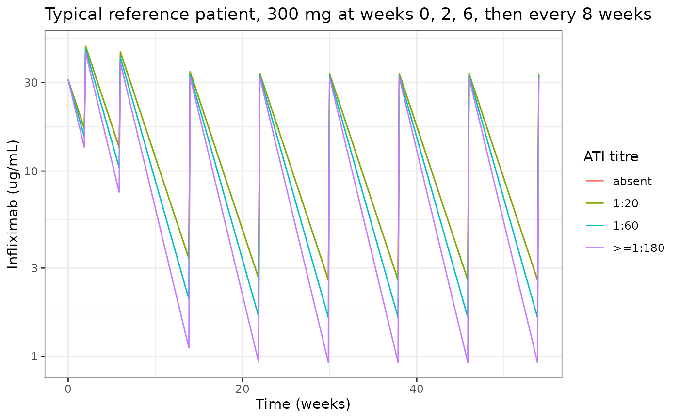
ATI titres of 1:60 and >= 1:180 raise clearance by 17% and 38%; the 1:20 class shares the reference clearance, so its curve overlies the ATI-absent one.
trough_typ <- sim_typ |>
  filter(time %in% c(13, 41, 97)) |>
  select(ati, time, Cc) |>
  mutate(week = (time + 1) / 7)

kel_ref <- 0.45 / 9.65
c_wk2_closed <- 300 / 9.65 * exp(-kel_ref * 13)
c_wk2_sim <- trough_typ$Cc[trough_typ$ati == "absent" & trough_typ$time == 13]
stopifnot(abs(c_wk2_sim / c_wk2_closed - 1) < 1e-4)

trough_typ |>
  select(-time) |>
  pivot_wider(names_from = week, values_from = Cc, names_prefix = "week_") |>
  rename(
    "ATI titre" = ati,
    "Trough week 2 (ug/mL)" = week_2,
    "Trough week 6 (ug/mL)" = week_6,
    "Trough week 14 (ug/mL)" = week_14
  ) |>
knitr::kable(digits = 2)| ATI titre | Trough week 2 (ug/mL) | Trough week 6 (ug/mL) | Trough week 14 (ug/mL) |
|---|---|---|---|
| absent | 16.96 | 13.42 | 3.38 |
| 1:20 | 16.96 | 13.42 | 3.38 |
| 1:60 | 15.30 | 10.45 | 2.04 |
| >=1:180 | 13.47 | 7.69 | 1.11 |
Virtual cohort and induction troughs
A cohort resembling Table 1 receives the dose mix of the study (14% 200 mg, 75% 300 mg, 11% 400 mg) at weeks 0, 2 and 6. Weight is drawn from a normal distribution with the Table 1 mean and SD truncated to its range, 24% of subjects are women, and baseline albumin is log-normal with the Table 1 median and IQR. Heights are 170 cm (SD 6) for men and 158 cm (SD 5) for women; see “Assumptions and deviations” for why the Table 1 height is not used. All subjects are ATI-absent, which is how the week-2 target was simulated in the paper.
set.seed(2024)
rxode2::rxSetSeed(2024)

n_sub <- 200
cohort <- tibble(
  id = seq_len(n_sub),
  SEXF = rbinom(n_sub, 1, 34 / 140),
  WT = pmin(pmax(rnorm(n_sub, 59.9, 10.8), 39), 80),
  HT = ifelse(SEXF == 1, rnorm(n_sub, 158, 5), rnorm(n_sub, 170, 6)),
  ALB = pmin(pmax(rlnorm(n_sub, log(38.3), 0.167), 27.5), 53.1),
  dose = sample(c(200, 300, 400), n_sub, replace = TRUE, prob = c(19, 105, 16) / 140),
  ADA_TITER = 0
) |>
  mutate(
    FFM = janmahasatian_ffm(WT, HT, SEXF),
    treatment = paste(dose, "mg")
  )

summary(cohort$FFM)
#>    Min. 1st Qu.  Median    Mean 3rd Qu.    Max.
#>   27.81   42.21   47.94   47.25   52.83   60.58

trough_days <- c(13.99, 41.99, 97.99)
ev_cohort <- bind_rows(
  expand_grid(cohort, time = c(0, 14, 42)) |>
    mutate(amt = dose, evid = 1L),
  expand_grid(cohort, time = sort(c(seq(0, 98, by = 1), trough_days))) |>
    mutate(amt = NA_real_, evid = 0L)
) |>
  mutate(cmt = "central") |>
  arrange(id, time, desc(evid))

sim_cohort <- rxode2::rxSolve(mod, events = ev_cohort, keep = "treatment") |>
  as.data.frame()
#> ℹ parameter labels from comments will be replaced by 'label()'
sim_cohort |>
  group_by(time) |>
  summarise(
    p05 = quantile(sim, 0.05),
    p50 = median(sim),
    p95 = quantile(sim, 0.95),
    .groups = "drop"
  ) |>
  ggplot(aes(time / 7, p50)) +
  geom_ribbon(aes(ymin = p05, ymax = p95), alpha = 0.25, fill = "purple") +
  geom_line() +
  geom_hline(yintercept = 20.08, linetype = "dashed", colour = "red") +
  labs(
    x = "Time (weeks)",
    y = "Infliximab (ug/mL)",
    title = "Simulated induction, Table 1-like cohort (median and 90% interval)",
    caption = "Compare with the early bins of Figure 4 of Zhu 2024. Dashed line: week-2 target 20.08 ug/mL."
  ) +
  theme_bw()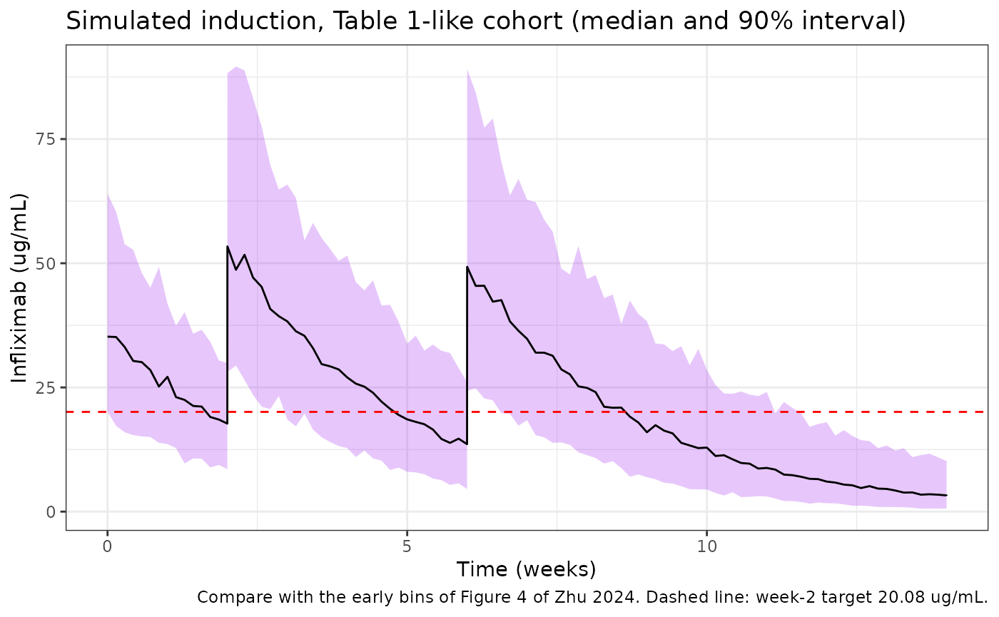
The paper reports median troughs only within the 43-patient remission cohort, split by outcome (Results, “Early induction IFX level”): week 2, 23.65 vs 16.96 ug/mL; week 6, 19.21 vs 11.18 ug/mL; week 14, 5.63 vs 2.21 ug/mL in patients with and without remission (29 and 14 patients). The simulated whole-cohort median is compared with the midpoint of the two group medians at weeks 2 and 6; it lands near the no-remission median, about 10-15% below the midpoint, and since two-thirds of the observed cohort were in remission the observed whole-cohort median is likely above the midpoint. Part of the gap plausibly reflects the assumed heights (a taller cohort has more fat-free mass and lower concentrations). Week 14 is not compared because the observed values include the ATI that a quarter of patients had developed by then (Figure 3A), which this ATI-absent simulation omits.
trough_sim <- sim_cohort |>
  filter(time %in% trough_days[1:2]) |>
  mutate(week = round((time + 0.01) / 7)) |>
  group_by(week) |>
  summarise(
    median_sim = median(sim),
    q25 = quantile(sim, 0.25),
    q75 = quantile(sim, 0.75),
    .groups = "drop"
  ) |>
  mutate(
    median_remission = c(23.65, 19.21),
    median_no_remission = c(16.96, 11.18)
  )

trough_sim |>
  rename(
    "Week" = week,
    "Simulated median (ug/mL)" = median_sim,
    "Simulated Q1" = q25,
    "Simulated Q3" = q75,
    "Observed median, remission" = median_remission,
    "Observed median, no remission" = median_no_remission
  ) |>
knitr::kable(digits = 2)| Week | Simulated median (ug/mL) | Simulated Q1 | Simulated Q3 | Observed median, remission | Observed median, no remission |
|---|---|---|---|---|---|
| 2 | 17.72 | 13.76 | 22.07 | 23.65 | 16.96 |
| 6 | 13.59 | 9.15 | 18.24 | 19.21 | 11.18 |
Replicating Figure 5: week-2 target attainment
Figure 5 shows the probability that the week-2 trough (immediately
before the second infusion) exceeds 20.08 ug/mL after a single induction
dose of 200-700 mg, by body weight (45-70 kg) and albumin (30, 35, 40
and 45 g/L), in ATI-absent patients, with 1,000 virtual patients per
point. The paper states neither the height nor the sex used to turn
weight into fat-free mass; the simulation below uses men (76% of the
cohort) 170 cm tall. The target is applied to the simulated observation
(sim, including residual error). The values in
fig5 were read from the figure by the maintainers.
fig5 <- tribble(
  ~ALB, ~dose, ~WT, ~pta_paper,
  30, 200, 45, 5, 30, 200, 50, 2, 30, 200, 55, 1,
  30, 300, 45, 40, 30, 300, 50, 32, 30, 300, 55, 26, 30, 300, 60, 11, 30, 300, 65, 18, 30, 300, 70, 14,
  30, 400, 45, 71, 30, 400, 50, 66, 30, 400, 55, 61, 30, 400, 60, 55, 30, 400, 65, 51, 30, 400, 70, 48,
  30, 500, 45, 86, 30, 500, 50, 84, 30, 500, 55, 81, 30, 500, 60, 77, 30, 500, 65, 74, 30, 500, 70, 72,
  30, 600, 55, 89, 30, 600, 60, 88, 30, 600, 65, 85, 30, 600, 70, 84,
  30, 700, 65, 92, 30, 700, 70, 91,
  35, 200, 45, 8, 35, 200, 50, 5, 35, 200, 55, 3,
  35, 300, 45, 46, 35, 300, 50, 37, 35, 300, 55, 33, 35, 300, 60, 26, 35, 300, 65, 22, 35, 300, 70, 19,
  35, 400, 45, 75, 35, 400, 50, 72, 35, 400, 55, 67, 35, 400, 60, 62, 35, 400, 65, 57, 35, 400, 70, 53,
  35, 500, 45, 89, 35, 500, 50, 86, 35, 500, 55, 83, 35, 500, 60, 81, 35, 500, 65, 79, 35, 500, 70, 76,
  35, 600, 55, 91, 35, 600, 60, 89, 35, 600, 65, 88, 35, 600, 70, 87,
  35, 700, 65, 93, 35, 700, 70, 93,
  40, 200, 45, 9, 40, 200, 50, 7, 40, 200, 55, 4,
  40, 300, 45, 52, 40, 300, 50, 45, 40, 300, 55, 39, 40, 300, 60, 32, 40, 300, 65, 27, 40, 300, 70, 22,
  40, 400, 45, 80, 40, 400, 50, 75, 40, 400, 55, 72, 40, 400, 60, 66, 40, 400, 65, 63, 40, 400, 70, 58,
  40, 500, 45, 91, 40, 500, 50, 89, 40, 500, 55, 86, 40, 500, 60, 84, 40, 500, 65, 82, 40, 500, 70, 80,
  40, 600, 55, 94, 40, 600, 60, 93, 40, 600, 65, 91, 40, 600, 70, 89,
  40, 700, 65, 96, 40, 700, 70, 97,
  45, 200, 45, 11, 45, 200, 50, 8, 45, 200, 55, 5,
  45, 300, 45, 55, 45, 300, 50, 50, 45, 300, 55, 43, 45, 300, 60, 36, 45, 300, 65, 31, 45, 300, 70, 26,
  45, 400, 45, 82, 45, 400, 50, 78, 45, 400, 55, 75, 45, 400, 60, 71, 45, 400, 65, 67, 45, 400, 70, 63,
  45, 500, 45, 92, 45, 500, 50, 90, 45, 500, 55, 88, 45, 500, 60, 86, 45, 500, 65, 84, 45, 500, 70, 82,
  45, 600, 55, 95, 45, 600, 60, 93, 45, 600, 65, 92, 45, 600, 70, 91,
  45, 700, 65, 96, 45, 700, 70, 95
)
nrow(fig5)
#> [1] 108
Each of the 108 scenarios is simulated with 200 virtual patients (the paper used 1,000), so a single simulated probability carries a Monte Carlo standard error of up to 3.5 percentage points.
n_per_arm <- 200
pta_ids <- fig5 |>
  mutate(arm = row_number()) |>
  expand_grid(rep = seq_len(n_per_arm)) |>
  mutate(
    id = row_number(),
    FFM = janmahasatian_ffm(WT, 170, 0),
    ADA_TITER = 0
  )

ev_pta <- bind_rows(
  pta_ids |> mutate(time = 0, amt = dose, evid = 1L),
  pta_ids |> mutate(time = 13.99, amt = NA_real_, evid = 0L)
) |>
  mutate(cmt = "central") |>
  arrange(id, time, desc(evid))

sim_pta <- rxode2::rxSolve(mod, events = ev_pta, keep = "arm") |>
  as.data.frame()
#> [====|====|====|====|====|====|====|====|====|====] 0:00:00

pta_sim <- sim_pta |>
  group_by(arm) |>
  summarise(pta_sim = 100 * mean(sim > 20.08), .groups = "drop")

pta_cmp <- fig5 |>
  mutate(arm = row_number()) |>
  left_join(pta_sim, by = "arm") |>
  mutate(diff = pta_sim - pta_paper)
pta_cmp |>
  pivot_longer(c(pta_paper, pta_sim), names_to = "source", values_to = "pta") |>
  mutate(
    source = recode(source, pta_paper = "Zhu 2024 Figure 5", pta_sim = "This model"),
    dose = factor(paste(dose, "mg"), levels = paste(seq(200, 700, 100), "mg")),
    ALB = paste("Albumin", ALB, "g/L")
  ) |>
  ggplot(aes(WT, pta, colour = dose, linetype = source, shape = source)) +
  geom_line() +
  geom_point() +
  geom_hline(yintercept = c(50, 80), colour = "grey50", linetype = "dotted") +
  facet_wrap(~ALB) +
  labs(
    x = "Body weight (kg)",
    y = "Probability of week-2 trough > 20.08 ug/mL (%)",
    colour = "Dose",
    linetype = NULL,
    shape = NULL,
    caption = "Replicates Figure 5 of Zhu 2024."
  ) +
  theme_bw()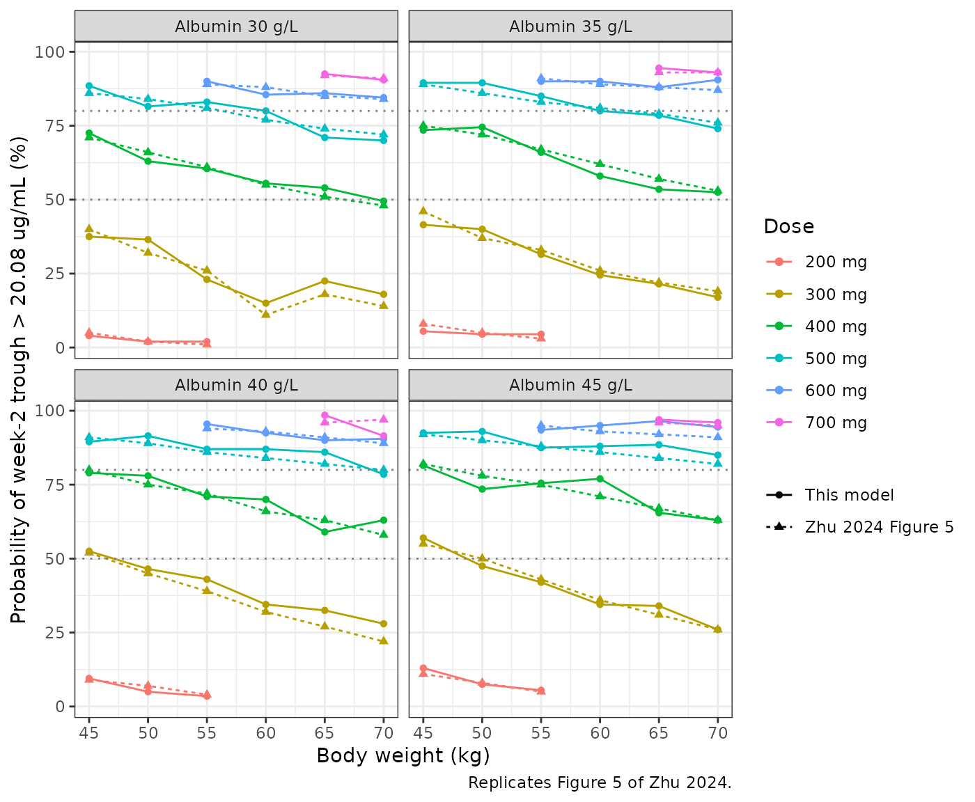
pta_cmp |>
  summarise(
    median_abs_diff = median(abs(diff)),
    p90_abs_diff = quantile(abs(diff), 0.9),
    max_abs_diff = max(abs(diff))
  ) |>
  rename(
    "Median |difference| (points)" = median_abs_diff,
    "90th percentile |difference|" = p90_abs_diff,
    "Max |difference|" = max_abs_diff
  ) |>
knitr::kable(digits = 1)| Median |difference| (points) | 90th percentile |difference| | Max |difference| |
|---|---|---|
| 1.5 | 4.2 | 6 |
# A wrong FFM exponent or reference moves the 70 kg points by 20-50
# percentage points (FFM taken equal to weight gives about 6% instead of
# the printed 22% at 300 mg, 70 kg, 40 g/L). With 200-subject Monte Carlo
# noise and figure reading, the 90th percentile of |difference| was 4.0-4.7
# over four seeds; single points reached 14.5.
stopifnot(
  abs(median(pta_cmp$diff)) < 5,
  quantile(abs(pta_cmp$diff), 0.9) < 12
)
The model reproduces Figure 5 across all four albumin panels. One printed point is out of line with its neighbours: 300 mg at 60 kg and 30 g/L reads 11% in the figure, below the 65 kg (18%) and 70 kg (14%) points, while clearance and volume change smoothly with weight; the model gives a value between the 55 kg and 65 kg points, as a smooth curve would.
Height sensitivity of the Figure 5 replication
Table 1 prints a mean height of 158.5 cm (SD 4.95, range 150-188), which is low for a cohort that is 76% male and hard to reconcile with an SD of 5 cm and a maximum of 188 cm. With 158.5 cm, FFM at a given weight is about 2 kg smaller and the typical week-2 trough about 4-5% higher:
typ_c14 <- function(dose, wt, alb, ht) {
  ffm <- janmahasatian_ffm(wt, ht, 0)
  cl <- 0.45 * (ffm / 56.1)^0.75 * (alb / 40)^-0.48
  v <- 9.65 * ffm / 56.1
  dose / v * exp(-cl / v * 13.99)
}
tibble(height_cm = c(158.5, 170)) |>
  mutate(
    ffm_at_45kg = janmahasatian_ffm(45, height_cm, 0),
    typical_c14_300mg_45kg_alb40 = typ_c14(300, 45, 40, height_cm),
    typical_c14_300mg_70kg_alb40 = typ_c14(300, 70, 40, height_cm)
  ) |>
  rename(
    "Height (cm)" = height_cm,
    "FFM at 45 kg, male (kg)" = ffm_at_45kg,
    "Typical week-2 trough, 300 mg, 45 kg (ug/mL)" = typical_c14_300mg_45kg_alb40,
    "Typical week-2 trough, 300 mg, 70 kg (ug/mL)" = typical_c14_300mg_70kg_alb40
  ) |>
knitr::kable(digits = 2)| Height (cm) | FFM at 45 kg, male (kg) | Typical week-2 trough, 300 mg, 45 kg (ug/mL) | Typical week-2 trough, 300 mg, 70 kg (ug/mL) |
|---|---|---|---|
| 158.5 | 39.54 | 21.64 | 17.50 |
| 170.0 | 41.54 | 20.78 | 16.59 |
That raises target attainment by a few percentage points, the same order as the Monte Carlo and digitisation noise in the comparison above, so Figure 5 cannot pin down the height the authors used. It does exclude using body weight in place of FFM, which changes the 70 kg points by 20-50 percentage points.
PKNCA: single induction dose
Single 200, 300 and 400 mg doses in the reference patient (FFM 56.1 kg, albumin 40 g/L, ATI absent), typical values. The paper reports no NCA, so the half-life is checked against the closed-form one-compartment value.
nca_ids <- tibble(id = 1:3, dose = c(200, 300, 400)) |>
  mutate(treatment = paste(dose, "mg"))
nca_times <- c(0, 0.04, 0.25, 1, 2, 4, 7, 14, 21, 28, 42, 56, 70, 84, 112)
ev_nca <- bind_rows(
  nca_ids |> mutate(time = 0, amt = dose, evid = 1L),
  expand_grid(nca_ids, time = nca_times) |> mutate(amt = NA_real_, evid = 0L)
) |>
  mutate(cmt = "central", FFM = 56.1, ALB = 40, ADA_TITER = 0) |>
  arrange(id, time, desc(evid))

sim_nca <- rxode2::rxSolve(mod_typ, events = ev_nca, keep = "treatment") |>
  as.data.frame() |>
  filter(!is.na(Cc))
#> ℹ omega/sigma items treated as zero: 'etalcl'
#> Warning: multi-subject simulation without without 'omega'

conc_obj <- PKNCA::PKNCAconc(sim_nca, Cc ~ time | treatment + id)
dose_obj <- PKNCA::PKNCAdose(
  nca_ids |> mutate(time = 0),
  dose ~ time | treatment + id
)
intervals <- data.frame(
  start = 0, end = Inf,
  cmax = TRUE, tmax = TRUE, aucinf.obs = TRUE, half.life = TRUE
)
nca_res <- PKNCA::pk.nca(PKNCA::PKNCAdata(conc_obj, dose_obj, intervals = intervals))

nca_tab <- as.data.frame(nca_res) |>
  filter(PPTESTCD %in% c("cmax", "aucinf.obs", "half.life")) |>
  select(treatment, PPTESTCD, PPORRES) |>
  pivot_wider(names_from = PPTESTCD, values_from = PPORRES)

nca_tab |>
  rename(
    "Dose" = treatment,
    "Cmax (ug/mL)" = cmax,
    "AUC0-inf (ug*day/mL)" = aucinf.obs,
    "t1/2 (day)" = half.life
  ) |>
knitr::kable(digits = 2)| Dose | Cmax (ug/mL) | t1/2 (day) | AUC0-inf (ug*day/mL) |
|---|---|---|---|
| 200 mg | 20.73 | 14.86 | 444.45 |
| 300 mg | 31.09 | 14.86 | 666.67 |
| 400 mg | 41.45 | 14.86 | 888.89 |
thalf_closed <- log(2) * 9.65 / 0.45
auc_closed <- nca_ids$dose / 0.45
stopifnot(
  all(abs(nca_tab$half.life / thalf_closed - 1) < 0.02),
  all(abs(nca_tab$aucinf.obs / auc_closed - 1) < 0.03)
)
The NCA half-life matches log(2) * V / CL = 14.9 days
and AUC0-inf matches dose / CL.
Assumptions and deviations
- Height and sex in the Figure 5 simulation. The paper simulates by body weight but the model is written in fat-free mass, and neither the height nor the sex behind the conversion is stated. Men 170 cm tall reproduce the figure; the Table 1 mean height of 158.5 cm gives target attainment a few percentage points higher (see the height-sensitivity section). The Table 1 height looks misprinted for a cohort that is 76% male, so the virtual cohort above uses sex-specific heights (170 cm for men, 158 cm for women) rather than the printed value.
- Residual error in the target-attainment simulation. The target is applied to the simulated observation including residual error. Applied to the individual prediction (IIV only), attainment is lower at the 70 kg points than the figure shows, so the paper’s simulation appears to include residual error even though the caption mentions only inter-patient variability.
- FFM reference value. The model normalises FFM to 56.1 kg. The Janmahasatian formula applied to the Table 1 demographics gives a median FFM nearer 47-50 kg, so 56.1 kg is not obviously the cohort median FFM; it is used as printed, and the Figure 5 replication confirms that the printed equations, with this reference, reproduce the authors’ simulations.
- Target value. The Results and the ROC analysis give 20.08 ug/mL; the Figure 5 caption and the Discussion print 20.8 ug/mL. The replication uses 20.08.
- Covariate time dependence. Albumin and ATI were screened as time-varying covariates and weight as both baseline and time-varying. The paper does not state which form of FFM entered the final model; the model accepts whatever FFM, ALB and ADA_TITER columns are supplied at each record.
-
ATI coding. ATI titres are reported as absent,
1:20, 1:60 and >= 1:180. The model takes the reciprocal dilution in
ADA_TITER(0 when absent) and applies the 1:60 factor for 60 <=ADA_TITER< 180 and the >= 1:180 factor from 180 upwards. Absent and 1:20 share the reference clearance, as in Eq. 4. - IIV. Table S5 reports IIV on CL as 25.1%, read here as a CV and converted to a log-normal variance of log(0.251^2 + 1) = 0.0611. No IIV on V was reported.
- Below-quantification samples were handled with the M5 method in the original fit; this has no bearing on simulation.
- Week-2 timing. Troughs are taken at day 13.99, just before the second infusion; doses are given as boluses because infusion durations were not reported, which has a negligible effect on troughs two weeks later.