Oncolytic virus + pembrolizumab QSP (Yamada 2025)
Source:vignettes/articles/Yamada_2025_oncolytic_virus_pembrolizumab.Rmd
Yamada_2025_oncolytic_virus_pembrolizumab.RmdThe paper
Yamada et al. (2025) used a multiple model-informed drug-development (MIDD) strategy to choose a first-in-human dosing regimen for an intratumorally injected oncolytic vaccinia virus carrying interleukin-7 and interleukin-12 genes (hIL-7/mIL-12-VV in mice, hIL-7/hIL-12-VV in humans) combined with an anti-PD-1 antibody (the murine surrogate RMP1-14, clinically pembrolizumab). The paper develops four models:
- a mouse preclinical QSP model (10 ODEs) calibrated to four CT26.WT tumour-growth experiments;
- a human clinical QSP model built by extending the Wang et al. 2020 immune-oncology platform with the oncolytic-virus mechanism;
- a mouse agent-based model (ABM); and
- a human ABM.
The two QSP models are ordinary-differential-equation systems and are packaged here:
Yamada_2025_oncolyticVirus_mouse_qspYamada_2025_oncolyticVirus_human_qsp
The two ABMs are agent-based cell-cycle simulations (Physiomics’ Virtual Tumour) whose tumour-growth engine is an ensemble of cell-cycle agents with a proprietary volume algorithm rather than an ODE system; they are not packaged (see Assumptions and deviations).
mod_mouse <- rxode2::rxode2(readModelDb("Yamada_2025_oncolyticVirus_mouse_qsp"))
mod_human <- rxode2::rxode2(readModelDb("Yamada_2025_oncolyticVirus_human_qsp"))
Population
Both models are deterministic mechanism models: the authors generated virtual subjects by sampling parameter ranges (preclinical fit / Latin hypercube sampling), not by fitting inter-individual variability or residual error, so the packaged models carry no etas and no error model.
-
Mouse QSP was calibrated in NONMEM to four CT26.WT
subcutaneous tumour-growth experiments in BALB/c mice (Exp1-Exp4, 19
conditions including 6 vehicle arms, 6-10 mice per arm; Supplementary
Table S1). Tumour volumes were converted to cell counts assuming
1e6cells/mm^3. Fourteen of the 28 parameters were estimated; the minimisation terminated before convergence and the authors used the terminated estimates (Supplementary Table S2). -
Human QSP inherits its immune-network parameters
from the Wang 2020 HER2-negative-breast-cancer model (Ref 4). 125
virtual-patient parameter sets were sampled from the Supplementary Table
S6 ranges; 100 reached a preselected baseline tumour diameter (uniform
1.0-4.5 cm) within an 8000-day untreated run-in that started from
1e6cancer cells. The viral infection rate constant was lowered relative to the mouse model to keep the single-agent objective response rate below 50%.
Source trace
| Model element | Source |
|---|---|
| Mouse QSP ODEs (virus, tumour Ni/I, nTeff, dTeff, PD-L1, anti-PD-1 depot/central, distant tumour) | Supplement eqs 1-10 |
Mouse QSP PD-L1 equation numerator (dTeff) |
Kosinsky 2018 (Ref 3) eq 16; Table S2 K_pdl
definition |
| Mouse QSP algebraic rules (TCD, DCm, Agsys, PD_L1free, ISC, IAR) | Supplementary Table S2 (Rules) |
Mouse QSP 28 parameters, per-experiment growth rate
r
|
Supplementary Table S2 |
| Mouse QSP baseline tumour volume (100 mm^3) | Supplementary Methods S1 (randomisation at > 100 mm^3) |
| Mouse dosing regimens | Supplementary Table S1 |
| Human QSP reactions R1-R158 | Supplementary Table S3 |
Human QSP rules (incl. V_T.C1 = Cuit + Cit,
IL7_act, IL12_act) |
Supplementary Table S4 |
| Human QSP fixed parameters, incl. pembrolizumab PK/binding and the oncolytic-virus block | Supplementary Table S5 |
| Human QSP virtual-population parameters (typical values used) | Supplementary Table S6 |
Human QSP parameters not tabulated by Yamada (durvalumab, ipilimumab
PK, k_C1_therapy) and initial species amounts |
Wang 2020 (Ref 4) supplement / SBML deposit |
Human run-in from 1e6 cells; dose volume by tumour
size; regimens |
Methods, “Human QSP Model Simulations” |
Mouse preclinical QSP
The mouse model describes an injected tumour
(tumour_volume, the sum of noninfected and infected cells)
and a distant noninjected tumour (tumour_volume_distant).
Virus is injected intratumorally (into virus, pfu) and the
anti-PD-1 antibody intraperitoneally (into mAbDep, nmol;
100 ug of a ~150 kDa antibody is 0.667 nmol). The tumour-growth rate
constant r was fitted separately for each experiment, so
each experiment is simulated with its own value.
mab_nmol <- 100e-6 / 150000 * 1e9 # 100 ug anti-PD-1 -> nmol
r_exp <- c(Exp1 = 0.36, Exp2 = 0.284, Exp3 = 0.348, Exp4 = 0.394)
mab_d1 <- c(1, 3, 7, 10, 15, 17, 20, 23, 28, 31)
mab_d7 <- c(7, 10, 15, 17)

design <- list(
  list(exp = "Exp1", arm = "vehicle", vd = 0, vdays = c(1, 3, 5), mdays = NULL),
  list(exp = "Exp1", arm = "2e4", vd = 2e4, vdays = c(1, 3, 5), mdays = NULL),
  list(exp = "Exp1", arm = "2e5", vd = 2e5, vdays = c(1, 3, 5), mdays = NULL),
  list(exp = "Exp1", arm = "2e6", vd = 2e6, vdays = c(1, 3, 5), mdays = NULL),
  list(exp = "Exp1", arm = "2e7", vd = 2e7, vdays = c(1, 3, 5), mdays = NULL),
  list(exp = "Exp2", arm = "vehicle", vd = 0, vdays = 1, mdays = NULL),
  list(exp = "Exp2", arm = "2e7 day1", vd = 2e7, vdays = 1, mdays = NULL),
  list(exp = "Exp2", arm = "2e7 day1, 8", vd = 2e7, vdays = c(1, 8), mdays = NULL),
  list(exp = "Exp2", arm = "2e7 day1, 15", vd = 2e7, vdays = c(1, 15), mdays = NULL),
  list(exp = "Exp3", arm = "vehicle", vd = 0, vdays = c(1, 3, 5), mdays = NULL),
  list(exp = "Exp3", arm = "2e6", vd = 2e6, vdays = c(1, 3, 5), mdays = NULL),
  list(exp = "Exp3", arm = "2e7", vd = 2e7, vdays = c(1, 3, 5), mdays = NULL),
  list(exp = "Exp4", arm = "vehicle", vd = 0, vdays = c(1, 3, 7), mdays = NULL),
  list(exp = "Exp4", arm = "2e7", vd = 2e7, vdays = c(1, 3, 7), mdays = NULL),
  list(exp = "Exp4", arm = "aPD1 (day1)", vd = 0, vdays = NULL, mdays = mab_d1),
  list(exp = "Exp4", arm = "aPD1 (day7)", vd = 0, vdays = NULL, mdays = mab_d7),
  list(exp = "Exp4", arm = "2e7 + aPD1 (day1)", vd = 2e7, vdays = c(1, 3, 7), mdays = mab_d1),
  list(exp = "Exp4", arm = "2e7 + aPD1 (day7)", vd = 2e7, vdays = c(1, 3, 7), mdays = mab_d7)
)

solve_mouse <- function(d, tmax = 21) {
  ev <- rxode2::et(seq(0, tmax, by = 0.25), cmt = "tumNi")
  if (d$vd > 0) {
    ev <- rxode2::et(ev, time = d$vdays, amt = d$vd, cmt = "virus")
  }
  if (!is.null(d$mdays)) {
    ev <- rxode2::et(ev, time = d$mdays[d$mdays <= tmax], amt = mab_nmol, cmt = "mAbDep")
  }
  s <- rxode2::rxSolve(mod_mouse, ev, params = c(r = r_exp[[d$exp]]),
                       method = "liblsoda", returnType = "data.frame")
  data.frame(exp = d$exp, arm = d$arm, time = s$time,
             injected = s$tumour_volume, distant = s$tumour_volume_distant)
}
mouse_sim <- dplyr::bind_rows(lapply(design, solve_mouse))
ggplot(mouse_sim, aes(time, injected, colour = arm)) +
  geom_line() +
  facet_wrap(~exp, scales = "free_y") +
  scale_y_log10() +
  labs(x = "Day after randomisation", y = "Injected tumour volume (mm^3)",
       colour = NULL,
       title = "Mouse QSP: injected tumour, Table S1 regimens (cf. Figure S2)")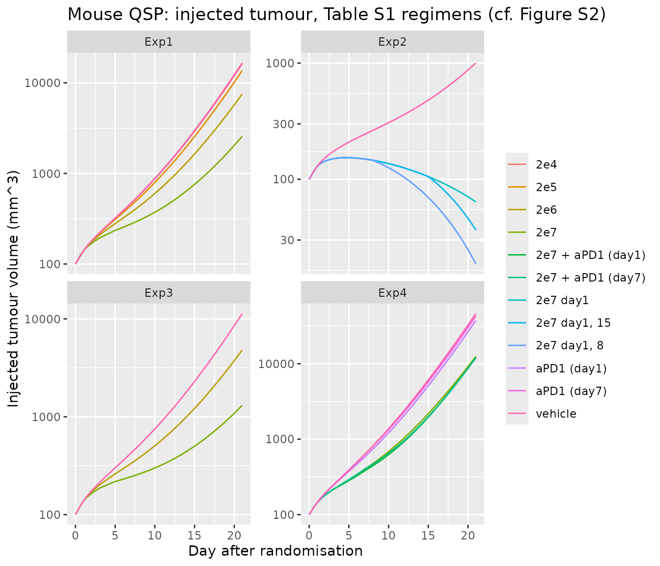
mouse_sim |>
  dplyr::filter(exp %in% c("Exp3", "Exp4")) |>
  tidyr::pivot_longer(c(injected, distant), names_to = "site",
                      values_to = "volume") |>
  ggplot(aes(time, volume, colour = arm, linetype = site)) +
  geom_line() +
  facet_wrap(~exp) +
  scale_y_log10() +
  labs(x = "Day after randomisation", y = "Tumour volume (mm^3)",
       colour = NULL, linetype = NULL,
       title = "Mouse QSP: injected vs distant tumour (cf. Figure S2)")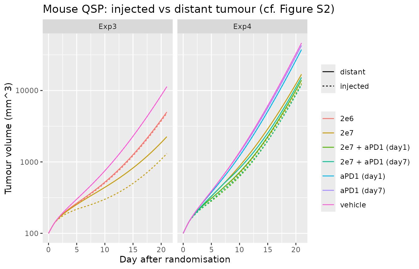
Volumes on day 14, when most vehicle arms are still within the measured range:
d14 <- mouse_sim |>
  dplyr::filter(time == 14) |>
  dplyr::select(exp, arm, injected, distant)
d14 |>
  dplyr::rename("Experiment" = exp, "Arm" = arm,
                "Injected (mm^3)" = injected, "Distant (mm^3)" = distant) |>
knitr::kable(digits = 0, caption = "Simulated tumour volume on day 14")| Experiment | Arm | Injected (mm^3) | Distant (mm^3) |
|---|---|---|---|
| Exp1 | vehicle | 2298 | 2298 |
| Exp1 | 2e4 | 2258 | 2258 |
| Exp1 | 2e5 | 1987 | 1992 |
| Exp1 | 2e6 | 1314 | 1358 |
| Exp1 | 2e7 | 642 | 980 |
| Exp2 | vehicle | 434 | 434 |
| Exp2 | 2e7 day1 | 112 | 154 |
| Exp2 | 2e7 day1, 8 | 81 | 142 |
| Exp2 | 2e7 day1, 15 | 112 | 154 |
| Exp3 | vehicle | 1802 | 1802 |
| Exp3 | 2e6 | 1001 | 1037 |
| Exp3 | 2e7 | 443 | 717 |
| Exp4 | vehicle | 4453 | 4453 |
| Exp4 | 2e7 | 1685 | 2232 |
| Exp4 | aPD1 (day1) | 3753 | 3753 |
| Exp4 | aPD1 (day7) | 4209 | 4209 |
| Exp4 | 2e7 + aPD1 (day1) | 1511 | 1741 |
| Exp4 | 2e7 + aPD1 (day7) | 1543 | 1957 |
v14 <- function(e, a, site = "injected") d14[[site]][d14$exp == e & d14$arm == a]

# Exp1: tumour-growth inhibition is ordered by virus dose.
exp1 <- vapply(c("vehicle", "2e4", "2e5", "2e6", "2e7"),
               function(a) v14("Exp1", a), numeric(1))
stopifnot(all(diff(exp1) < 0))

# Exp3: the systemic dTeff pool slows the distant tumour as well, but less
# than the injected one.
stopifnot(
  v14("Exp3", "2e7", "distant") < v14("Exp3", "vehicle", "distant"),
  v14("Exp3", "2e7", "distant") > v14("Exp3", "2e7", "injected")
)

# Exp4: anti-PD-1 adds to the virus effect in both schedules.
stopifnot(
  v14("Exp4", "2e7 + aPD1 (day1)") < v14("Exp4", "2e7"),
  v14("Exp4", "2e7 + aPD1 (day7)") < v14("Exp4", "2e7")
)
The packaged model reproduces the dose-ordered response at the
injected tumour and a weaker abscopal effect at the distant tumour. With
the published parameter values the anti-PD-1-enhanced virus clearance is
a small effect (Imax = 0.139, a 13.9% increase), so in Exp4
the immune benefit of the extra anti-PD-1 doses in the simultaneous arm
(10 doses from day 1, against 4 from day 7) outweighs it: on day 14 the
simultaneous arm is slightly smaller than the sequential arm at both
sites. The paper reports that its model favoured the sequential regimen
(Results, “Mouse QSP Modeling”); Figure S2, which shows that fit, is not
reproduced here, and the parameters were not tuned to recover it.
Anti-PD-1 antibody pharmacokinetics (PKNCA)
The anti-PD-1 arm adds a first-order depot-to-central PK model. The serum PK of a single 100 ug intraperitoneal dose is summarised with PKNCA.
ev_pk <- rxode2::et(seq(0, 30, by = 0.25), cmt = "mAbC") |>
  rxode2::et(time = 0, amt = mab_nmol, cmt = "mAbDep")
pk <- rxode2::rxSolve(mod_mouse, ev_pk, returnType = "data.frame")
pk_in <- pk |>
  dplyr::mutate(conc = mAbC / 0.003, id = 1L, # nmol / Vd (L) = nM
                treatment = "anti-PD-1 100 ug IP") |>
  dplyr::filter(!is.na(conc))

o_conc <- PKNCA::PKNCAconc(pk_in, conc ~ time | treatment + id)
o_dose <- PKNCA::PKNCAdose(
  data.frame(time = 0, dose = mab_nmol, id = 1L,
             treatment = "anti-PD-1 100 ug IP"),
  dose ~ time | treatment + id
)
res <- PKNCA::pk.nca(PKNCA::PKNCAdata(
  o_conc, o_dose,
  intervals = data.frame(start = 0, end = 30, cmax = TRUE, tmax = TRUE,
                         auclast = TRUE, half.life = TRUE)
))
nca <- as.data.frame(res$result)
nca |>
  dplyr::select(PPTESTCD, PPORRES) |>
  dplyr::rename("NCA parameter" = PPTESTCD, "Value" = PPORRES) |>
knitr::kable(digits = 3, caption = "Anti-PD-1 serum NCA (mouse QSP, nM and days)")| NCA parameter | Value |
|---|---|
| auclast | 1455.866 |
| cmax | 205.957 |
| tmax | 0.500 |
| tlast | 30.000 |
| lambda.z | 0.150 |
| r.squared | 1.000 |
| adj.r.squared | 1.000 |
| lambda.z.time.first | 0.750 |
| lambda.z.time.last | 30.000 |
| lambda.z.n.points | 118.000 |
| clast.pred | 2.516 |
| half.life | 4.621 |
| span.ratio | 6.330 |
Human clinical QSP
The human model grows a tumour from 1e6 cancer cells;
therapy starts once the tumour reaches its baseline diameter, with the
node values at that moment as the patient’s initial conditions (as in
the paper). One untreated run-in gives the initial conditions for four
typical patients at baseline diameters of 1.5, 2.5, 3.5 and 4.4 cm, one
in each of the paper’s dose-volume bands (1, 2, 4 and 6 mL of virus
suspension). The virus dose in pfu is the concentration (pfu/mL) times
that volume.
human_ctl <- list(method = "cvode", maxsteps = 5e5, atol = 1e-9, rtol = 1e-9)
solve_human <- function(ev, inits = NULL) {
  rxode2::rxSolve(mod_human, ev, inits = inits, method = human_ctl$method,
                  maxsteps = human_ctl$maxsteps, atol = human_ctl$atol,
                  rtol = human_ctl$rtol, returnType = "data.frame")
}
runin <- solve_human(rxode2::et(seq(0, 3000, by = 2), cmt = "q_V_T_Cit"))

patients <- data.frame(
  patient = c("1.5 cm", "2.5 cm", "3.5 cm", "4.4 cm"),
  base_cm = c(1.5, 2.5, 3.5, 4.4),
  dose_mL = c(1, 2, 4, 6)
)
patients$t_base <- vapply(patients$base_cm, function(b) {
  runin$time[which(runin$tumour_diameter >= b)[1]]
}, numeric(1))
knitr::kable(
  patients |>
    dplyr::rename("Patient" = patient, "Baseline diameter (cm)" = base_cm,
                  "Virus volume (mL)" = dose_mL,
                  "Run-in time to baseline (days)" = t_base),
  caption = "Typical patients taken from the untreated run-in"
)| Patient | Baseline diameter (cm) | Virus volume (mL) | Run-in time to baseline (days) |
|---|---|---|---|
| 1.5 cm | 1.5 | 1 | 884 |
| 2.5 cm | 2.5 | 2 | 1094 |
| 3.5 cm | 3.5 | 4 | 1234 |
| 4.4 cm | 4.4 | 6 | 1328 |
Arms: virus alone at 1e7, 1e8 or 5e8 pfu/mL every 2 weeks (Figure S3), and 5e8 pfu/mL plus pembrolizumab 400 mg every 6 weeks starting 0, 1, 2 or 4 weeks after the first virus dose (H-0W to H-4W, Figure 4).
pembro_nmol <- 400 / 149000 * 1e6 # 400 mg pembrolizumab, MW ~149 kDa -> nmol
arms <- data.frame(
  arm = c("untreated", "1e7", "1e8", "5e8", "H-0W", "H-1W", "H-2W", "H-4W"),
  conc = c(0, 1e7, 1e8, 5e8, 5e8, 5e8, 5e8, 5e8),
  pembro_start = c(NA, NA, NA, NA, 0, 7, 14, 28)
)
horizon <- 400
run_arm <- function(p, a) {
  inits <- unlist(runin[runin$time == patients$t_base[p], mod_human$state])
  ev <- rxode2::et(seq(0, horizon, by = 5), cmt = "q_V_T_Cit")
  if (arms$conc[a] > 0) {
    ev <- rxode2::et(ev, time = seq(0, horizon, by = 14),
                     amt = arms$conc[a] * patients$dose_mL[p],
                     cmt = "q_V_T_Virus_T")
  }
  if (!is.na(arms$pembro_start[a])) {
    ev <- rxode2::et(ev, time = seq(arms$pembro_start[a], horizon, by = 42),
                     amt = pembro_nmol, cmt = "q_V_C_pembro")
  }
  s <- solve_human(ev, inits = inits)
  data.frame(patient = patients$patient[p], arm = arms$arm[a], time = s$time,
             diameter = s$tumour_diameter,
             pct_change = 100 * (s$tumour_diameter / s$tumour_diameter[1] - 1))
}
human_sim <- dplyr::bind_rows(lapply(seq_len(nrow(patients)), function(p) {
  dplyr::bind_rows(lapply(seq_len(nrow(arms)), function(a) run_arm(p, a)))
}))
human_sim$arm <- factor(human_sim$arm, levels = arms$arm)
ggplot(human_sim, aes(time, pct_change, colour = arm)) +
  geom_line() +
  geom_hline(yintercept = -30, linetype = "dashed") +
  facet_wrap(~patient) +
  coord_cartesian(ylim = c(-100, 150)) +
  labs(x = "Day after treatment start",
       y = "Change in tumour diameter from baseline (%)", colour = NULL,
       title = "Human QSP: virus alone and with pembrolizumab (cf. Figures 4 and S3)")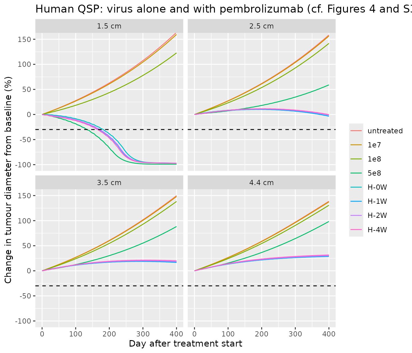
resp <- human_sim |>
  dplyr::filter(time %in% c(100, 365)) |>
  dplyr::select(patient, arm, time, pct_change) |>
  tidyr::pivot_wider(names_from = time, values_from = pct_change,
                     names_prefix = "day_")
resp |>
  dplyr::rename("Patient" = patient, "Arm" = arm,
                "Day 100 change (%)" = day_100,
                "Day 365 change (%)" = day_365) |>
  knitr::kable(digits = 1,
caption = "Change in tumour diameter from baseline (RECIST response at <= -30%)")| Patient | Arm | Day 100 change (%) | Day 365 change (%) |
|---|---|---|---|
| 1.5 cm | untreated | 27.7 | 142.5 |
| 1.5 cm | 1e7 | 26.7 | 138.8 |
| 1.5 cm | 1e8 | 18.4 | 105.7 |
| 1.5 cm | 5e8 | -18.4 | -99.1 |
| 1.5 cm | H-0W | -8.3 | -96.7 |
| 1.5 cm | H-1W | -10.7 | -96.8 |
| 1.5 cm | H-2W | -10.5 | -96.8 |
| 1.5 cm | H-4W | -12.1 | -96.9 |
| 2.5 cm | untreated | 27.3 | 138.6 |
| 2.5 cm | 1e7 | 26.9 | 136.8 |
| 2.5 cm | 1e8 | 23.3 | 123.4 |
| 2.5 cm | 5e8 | 7.4 | 49.6 |
| 2.5 cm | H-0W | 8.6 | 3.0 |
| 2.5 cm | H-1W | 7.9 | 1.1 |
| 2.5 cm | H-2W | 8.4 | 3.0 |
| 2.5 cm | H-4W | 8.3 | 3.8 |
| 3.5 cm | untreated | 27.0 | 132.2 |
| 3.5 cm | 1e7 | 26.7 | 130.8 |
| 3.5 cm | 1e8 | 24.0 | 121.6 |
| 3.5 cm | 5e8 | 12.5 | 75.8 |
| 3.5 cm | H-0W | 11.6 | 18.6 |
| 3.5 cm | H-1W | 11.3 | 17.9 |
| 3.5 cm | H-2W | 11.8 | 19.5 |
| 3.5 cm | H-4W | 12.1 | 20.8 |
| 4.4 cm | untreated | 26.5 | 123.9 |
| 4.4 cm | 1e7 | 26.3 | 122.7 |
| 4.4 cm | 1e8 | 24.3 | 116.3 |
| 4.4 cm | 5e8 | 15.5 | 85.9 |
| 4.4 cm | H-0W | 13.6 | 28.5 |
| 4.4 cm | H-1W | 13.4 | 28.1 |
| 4.4 cm | H-2W | 13.9 | 29.4 |
| 4.4 cm | H-4W | 14.4 | 30.8 |
chg <- function(p, a, day = "day_365") resp[[day]][resp$patient == p & resp$arm == a]

for (p in patients$patient) {
  # virus monotherapy is ordered by dose at every baseline size
  mono <- vapply(c("untreated", "1e7", "1e8", "5e8"), function(a) chg(p, a),
                 numeric(1))
  stopifnot(all(diff(mono) < 0))
  # the four pembrolizumab schedules end within 5 percentage points of each
  # other by day 365 (paper: no obvious difference between schedules)
  combo <- vapply(c("H-0W", "H-1W", "H-2W", "H-4W"), function(a) chg(p, a),
                  numeric(1))
  stopifnot(diff(range(combo)) < 5)
}

# Adding pembrolizumab improves day-365 control over the high virus dose alone
# for the patients who do not respond to the virus alone.
for (p in c("2.5 cm", "3.5 cm", "4.4 cm")) {
  stopifnot(chg(p, "H-0W") < chg(p, "5e8") - 20)
}

# The infected-cell / virus cascade engages after a single dose: infected
# cells appear (lysed within hours, Delta_I = 57.4/day, so the infected
# fraction stays small) and the cancer-cell count falls over the first days.
tx <- solve_human(
  rxode2::et(seq(0, 28, by = 1), cmt = "q_V_T_Cit") |>
    rxode2::et(time = 0, amt = 5e8, cmt = "q_V_T_Virus_T"),
  inits = unlist(runin[runin$time == patients$t_base[1], mod_human$state])
)
stopifnot(
  max(tx$infected_fraction) > 1e-4,
  min(tx$cancer_cells[tx$time <= 7]) < 0.95 * tx$cancer_cells[1]
)
The paper’s virtual population gave objective response rates of 0%, 2% and 22% for virus alone at 1e7, 1e8 and 5e8 pfu/mL and 48% for every combination schedule at day 365. The four typical patients here follow the same pattern: virus alone is dose-ordered and shrinks only the smallest tumour, while pembrolizumab adds a large benefit by day 365 for the larger tumours and the four schedules end within a few percentage points of each other. At day 100 the paper ranked the schedules 1 week >= 0 weeks > 2 weeks > 4 weeks by response rate; for the typical 1.5 cm patient here the early differences are within a few percentage points and the later starts are marginally better, because the pembrolizumab-enhanced virus clearance acts before the immune benefit builds up. A response rate needs the Table S6 virtual population, which is not reproduced (see below).
Pembrolizumab pharmacokinetics (PKNCA)
base1 <- unlist(runin[runin$time == patients$t_base[1], mod_human$state])
pk_h <- solve_human(
  rxode2::et(seq(0, 42, by = 0.5), cmt = "q_V_C_pembro") |>
    rxode2::et(time = 0, amt = pembro_nmol, cmt = "q_V_C_pembro"),
  inits = base1
)
pk_hin <- pk_h |>
  dplyr::mutate(conc = Cc_pembrolizumab, id = 1L,
                treatment = "pembrolizumab 400 mg IV") |>
  dplyr::filter(!is.na(conc))
o_conc_h <- PKNCA::PKNCAconc(pk_hin, conc ~ time | treatment + id)
o_dose_h <- PKNCA::PKNCAdose(
  data.frame(time = 0, dose = pembro_nmol, id = 1L,
             treatment = "pembrolizumab 400 mg IV"),
  dose ~ time | treatment + id
)
res_h <- PKNCA::pk.nca(PKNCA::PKNCAdata(
  o_conc_h, o_dose_h,
  intervals = data.frame(start = 0, end = 42, cmax = TRUE, tmax = TRUE,
                         auclast = TRUE, half.life = TRUE)
))
nca_h <- as.data.frame(res_h$result)
nca_h |>
  dplyr::select(PPTESTCD, PPORRES) |>
  dplyr::rename("NCA parameter" = PPTESTCD, "Value" = PPORRES) |>
knitr::kable(digits = 3, caption = "Pembrolizumab plasma NCA (human QSP, nM and days)")| NCA parameter | Value |
|---|---|
| auclast | 6305.782 |
| cmax | 447.427 |
| tmax | 0.000 |
| tlast | 42.000 |
| lambda.z | 0.016 |
| r.squared | 1.000 |
| adj.r.squared | 1.000 |
| lambda.z.time.first | 12.000 |
| lambda.z.time.last | 42.000 |
| lambda.z.n.points | 61.000 |
| clast.pred | 95.107 |
| half.life | 42.639 |
| span.ratio | 0.704 |
Assumptions and deviations
- The two agent-based models are not packaged. The mouse and human ABMs are Physiomics’ Virtual Tumour, an agent-based cell-cycle simulation whose tumour volume comes from a proprietary algorithm; it is not an ODE system and cannot be expressed in rxode2. Only the immune-system component of the ABM is an ODE set (Supplement eqs 1-12, Table S7), and it is driven by the cell count from the agent engine, so it is not a standalone model either.
-
Mouse QSP PD-L1 equation. Supplement eq 6 is
printed with
PDL1in the numerator of the saturable term. The source model (Kosinsky 2018, Ref 3, eq 16) and the definition ofK_pdl(“sensitivity of PD-L1 expression up-regulation to dTeff count”, in cells) show that the numerator is the differentiated-effector-T-cell count; the packaged model usesdTeff / (dTeff + K_pdl). Eq 2 likewise printsT_efffor the killing term, which isdT_effin eqs 3 and 10 and in the source model. -
Mouse QSP eradication threshold. The infection flux
V_beta * Virus * Tum_ni / Tum_tot / 1e6does not shrink with tumour size while noninfected cells dominate, so the injected tumour reaches zero in finite time and theTum_ni / Tum_totandTum_i / Tum_totratios become infinitely stiff (the solver fails, for example, in the Exp2 day 1 + 8 arm). Below one tumour cell (1e-6mm^3) the packaged model freezes the two injected-tumour volumes and floors the ratio denominators at one cell. This changes nothing while the tumour is larger than one cell. -
Mouse QSP growth rate.
rwas fitted per experiment (0.36, 0.284, 0.348 and 0.394 1/day for Exp1-Exp4). The model default is the Exp1 value; this vignette overridesrfor each experiment. - Mouse QSP control virus. The unmodified control virus (Exp1) has no IL-7 or IL-12 genes, but the model ties IL-7 and IL-12 stimulation to infected cells, so it cannot distinguish the two viruses; the control-virus arm is not simulated.
- Mouse QSP baseline and antibody dose. Mice were randomised when the tumour exceeded 100 mm^3; the injected and distant tumours start at 100 mm^3 with the immune and virus states at rest. The 100 ug anti-PD-1 dose is converted to nmol with an assumed molecular weight of 150 kDa.
- Mouse QSP fit did not converge. The NONMEM minimisation terminated before convergence and the authors used the terminated estimates; the packaged values are those estimates.
-
Human QSP is an extension of Wang 2020. The immune
network, its parameters and the initial species amounts are inherited
from the Wang 2020 model (Ref 4), packaged separately as
Wang_2020_entinostat_nivolumab_ipilimumab_qsp. The nivolumab arm is replaced by pembrolizumab (Table S5 parameters); the anti-PD-L1 (durvalumab), anti-CTLA-4 (ipilimumab) and entinostat modules are carried over but not dosed in this paper. Values are converted to the model’s counts/litre/dm^2/day system as in the Wang 2020 translation; eachini()line’s comment records the tabulated value and unit. Where Yamada’s tables differ from Wang 2020, Yamada’s value is used (k_C1_growth= 0.0075 1/day from Table S6;IC50_ENT_ArgI= 3.74e-7 M from Table S5). Parameters Yamada does not tabulate (durvalumab and ipilimumab PK,k_C1_therapy) and the initial species amounts come from Wang 2020. -
Human QSP run-in. The untreated run-in starts from
1e6cancer cells (Methods), not from the single cell of the Wang 2020 platform. Yamada’s Table S5 still lists the Wang pre-treatment diameter of 0.1 cm, which is not used. -
Human QSP virus units.
Virus_Tis held in molecule-equivalents, the unit of the Table S5 virus parameters (Alphain molecule/cell,Beta_infectin cell/day/molecule); one pfu is taken as one molecule-equivalent, as in the mouse model, where the same parameters are in pfu. The dose in pfu is the concentration times the tumour-size-dependent volume (Methods). -
Human QSP C2 tracker. Table S3 reaction 155 defines
a cancer-cell tracker
V_T.C2without infection, while Table S4 also lists the ruleV_T.C2 = V_T.Cuit.C2feeds back on nothing; the packaged model integrates reaction 155 as printed. -
Human QSP virtual population. The paper sampled 15
parameters from the Table S6 distributions by Latin hypercube; some
entries are ambiguous as printed (the lognormal
k_C1_growthhas “mean 0.0075, SD 1”; thek_cln_ENTrange is given as [6e-4, 1.22e-4]). The packaged model carries the typical values, and this vignette uses four typical patients at different baseline diameters rather than the virtual population, so it checks the pattern of response, not the published response rates. - No NCA was reported in the paper for either antibody; the PKNCA sections check the antibody PK sub-models against their own parameters.