Empagliflozin in paediatric type 2 diabetes (Rascher 2025)
Source:vignettes/articles/Rascher_2025_empagliflozin.Rmd
Rascher_2025_empagliflozin.RmdModel and source
Rascher et al. (2025) re-estimated the adult empagliflozin population PK and HbA1c exposure-response models (Baron 2016) on the paediatric DINAMO trial in a Bayesian (NUTS) framework. The analysis was sequential: the popPK model was fitted first, each patient’s steady-state AUC was computed as daily dose / individual CL/F, and that AUC then drove the HbA1c model. The package therefore ships two models:
-
Rascher_2025_empagliflozin– two-compartment popPK with sequential zero-order / first-order absorption. -
Rascher_2025_empagliflozin_hba1c– indirect-response HbA1c model driven by theAUC_EMPAcovariate.
mod_pk <- rxode2::rxode(readModelDb("Rascher_2025_empagliflozin"))
#> ℹ parameter labels from comments will be replaced by 'label()'
mod_pd <- rxode2::rxode(readModelDb("Rascher_2025_empagliflozin_hba1c"))
#> ℹ parameter labels from comments will be replaced by 'label()'
#> Warning: some etas defaulted to non-mu referenced, possible parsing error: etadp_slope
#> as a work-around try putting the mu-referenced expression on a simple line- Citation: Rascher J, Cheng S, Johnston C, Haertter S, Marquard J, Tartakovsky I, Laffel L, Wojtyniak J-G. Pharmacokinetics and pharmacodynamics of empagliflozin in paediatric patients aged 10-17 years with type 2 diabetes mellitus. Br J Clin Pharmacol. 2025;91(8):2390-2400. doi:10.1002/bcp.70096.
- PK description: Population pharmacokinetic model for oral empagliflozin in paediatric patients aged 10-17 years with type 2 diabetes mellitus (DINAMO trial). Two-compartment model with sequential zero-order (duration D1) then first-order (ka) absorption and linear elimination, re-estimated in a Bayesian (NUTS) framework from the adult Baron 2016 structure. Fixed allometric weight scaling (exponent 0.75 on CL/F and Q/F, 1 on V2/F and V3/F, reference 70 kg); power eGFR effect on CL/F (eGFR truncated at 120 mL/min/1.73 m^2, reference 90); multiplicative Black, Asian and female effects on CL/F. IIV on CL/F only.
- PD description: Exposure-response (indirect response) model for HbA1c in paediatric patients aged 10-17 years with type 2 diabetes mellitus treated with empagliflozin or placebo (DINAMO trial). Steady-state empagliflozin AUC (AUC_EMPA, from the companion Rascher_2025_empagliflozin popPK) inhibits HbA1c synthesis kin through an Imax function with AUC50 fixed at 703 nmol*h/L; kin rises by a zero-order disease-progression rate in patients on background insulin. Covariates: insulin co-therapy on baseline HbA1c and on progression; eGFR (truncated at 120) and observed baseline HbA1c power effects on Imax. Correlated IIV on baseline and progression.
- Article: https://doi.org/10.1002/bcp.70096 (open access, PMC12304805)
Population
DINAMO randomised young people aged 10-17 years with type 2 diabetes. The PK analysis used 223 quantifiable concentrations from 74 patients on empagliflozin 10 mg (n = 46), 25 mg (n = 16) or 10 mg re-randomised to 25 mg (n = 12) (Table 1). Table S2 gives a median weight of 90.0 kg (42.5-169), median age 14.5 years (10-17) and median eGFR of 125 mL/min/1.73 m^2 (89.7-241, Zappitelli equation); Table S1 gives 62.2% female, 50.0% White, 32.4% Black and 5.4% Asian. The HbA1c analysis used 394 observations from 103 patients: placebo (n = 51), empagliflozin 10 mg (n = 39) and 10 mg then 25 mg from week 15 (n = 13). 49.4% had background insulin and 90.3% background metformin (Results, Table 2).
str(mod_pk$population[c("n_subjects", "age_range", "weight_range", "sex_female_pct")])
#> List of 4
#>  $ n_subjects    : int 74
#>  $ age_range     : chr "10-17 years (median 14.5; Table S2)"
#>  $ weight_range  : chr "42.5-169 kg (median 90.0; Table S2)"
#>  $ sex_female_pct: num 62.2
str(mod_pd$population[c("n_subjects", "dose_range", "co_medication")])
#> List of 3
#>  $ n_subjects   : int 103
#>  $ dose_range   : chr "Placebo (n = 51); empagliflozin 10 mg weeks 1-26 (n = 39) or 10 mg weeks 1-14 then 25 mg weeks 15-26 (n = 13), "| __truncated__
#>  $ co_medication: chr "Insulin at baseline 51 patients (49.4%); metformin at baseline 93 patients (90.3%)."
Source trace
The covariate equations and the parameter-number mapping come from the supplement (“Equations for final PK/PD model parameters” and the CL/F equation), which carries them as images.
| Item | Value | Source |
|---|---|---|
| CL/F (male, non-Black, non-Asian, eGFR 90, 70 kg) | 6.74 L/h | Table 3; Supplement CL/F equation |
| V2/F, Q/F, V3/F | 4.12 L, 5.51 L/h, 71.7 L | Table 3 |
| ka, D1 | 0.239 1/h, 0.326 h | Table 3 |
| Allometric exponents (reference 70 kg) | 0.75 clearances, 1 volumes (fixed) | Methods ‘PopPK’; Supplement WT_CL = (WT/70)^theta |
| eGFR on CL/F | (min(eGFR, 120)/90)^0.407 | Table 3; Supplement EGFR_CL and truncation note |
| Black / Asian / female on CL/F | 0.897 / 0.934 / 1.19 | Table 3 (exp(theta)); Supplement CL/F equation |
| IIV CL/F | 33.3% CV -> omega^2 0.1052 | Table 3 and footnote |
| Residual error | 47.4% proportional + 1.67 nmol/L additive | Table 3 Sigma 1,1 and 2,2 |
| Sequential zero-/first-order absorption, 2-compartment | ODE | Methods ‘PopPK’ |
| kout | 0.0489 1/day | Table 4 |
| BASE (no insulin) | 7.35 % | Table 4 |
| Insulin effect on BASE | x 1.15 | Table 4 INS BASE; Supplement BASE equation |
| PROG | 5.64e-07 %/h/h, insulin only, + eta/100000 | Table 4; Supplement PROG equation |
| Imax (typical) | expit(theta 4) = 0.101 | Table 4; Supplement IMAX_TV |
| eGFR / baseline HbA1c on Imax | (min(eGFR,120)/90)^1.03, (HbA1c/7.9)^2.04 | Table 4; Supplement Imax text |
| AUC50 | 703 nmol*h/L (fixed) | Table 4; Methods ‘ER analyses’ |
| IIV BASE, PROG, covariance | 16.1% CV, 7.35, 0.00112 | Table 4 |
| Residual error HbA1c | SD 0.0632 on log scale | Table 4 Sigma 1,1 |
| dHbA1c/dt = kin (1 - INH) - kout HbA1c; dkin/dt = PROG | ODE | Methods ‘ER analyses’ equations |
| AUCss = dose / individual CL/F | covariate | Methods ‘PopPK’, last paragraph |
Pharmacokinetics
Virtual cohort
200 virtual patients per dose (10 mg and 25 mg once daily), with weight, eGFR, sex and race drawn to match Tables S1 and S2. Weight and eGFR are log-normal around the DINAMO medians, truncated to the observed ranges.
set.seed(2025)
rxode2::rxSetSeed(2025)
n_arm <- 200
make_cov <- function(n, id0) {
  race <- sample(c("other", "black", "asian"), n, replace = TRUE, prob = c(0.622, 0.324, 0.054))
  data.frame(
    id = id0 + seq_len(n),
    WT = pmin(pmax(exp(rnorm(n, log(90), 0.27)), 42.5), 169),
    CRCL = pmin(pmax(exp(rnorm(n, log(125), 0.18)), 89.7), 241),
    SEXF = rbinom(n, 1, 0.622),
    RACE_BLACK = as.integer(race == "black"),
    RACE_ASIAN = as.integer(race == "asian")
  )
}
cohort <- rbind(
  cbind(make_cov(n_arm, 0), dose = 10),
  cbind(make_cov(n_arm, n_arm), dose = 25)
) |>
  mutate(treatment = paste(dose, "mg QD"))

tau <- 24
n_dose <- 10
t_last <- (n_dose - 1) * tau
obs_t <- sort(unique(c(seq(0, 24, by = 0.25), t_last + seq(0, 24, by = 0.25))))

# rate = -2 makes rxode2 infuse each dose into the depot over the modelled D1.
ev_pk <- bind_rows(
  cohort |>
    tidyr::crossing(time = (0:(n_dose - 1)) * tau) |>
    mutate(amt = dose, evid = 1L, cmt = "depot", rate = -2),
  cohort |>
    tidyr::crossing(time = obs_t) |>
    mutate(amt = 0, evid = 0L, cmt = "central", rate = 0)
) |>
  arrange(id, time, desc(evid))

sim_pk <- rxode2::rxSolve(mod_pk, events = ev_pk, returnType = "data.frame",
                          keep = "treatment")
sim_pk <- left_join(sim_pk, select(cohort, id, dose), by = "id")
Concentration-time profiles at steady state
sim_pk |>
  filter(time >= t_last) |>
  group_by(treatment, tad = time - t_last) |>
  summarise(med = median(Cc), lo = quantile(Cc, 0.05), hi = quantile(Cc, 0.95), .groups = "drop") |>
  ggplot(aes(tad, med, colour = treatment, fill = treatment)) +
  geom_ribbon(aes(ymin = lo, ymax = hi), alpha = 0.2, colour = NA) +
  geom_line() +
  labs(x = "Time after dose (h)", y = "Empagliflozin (nmol/L)",
       title = "Simulated steady-state profiles (median, 5th-95th percentiles)")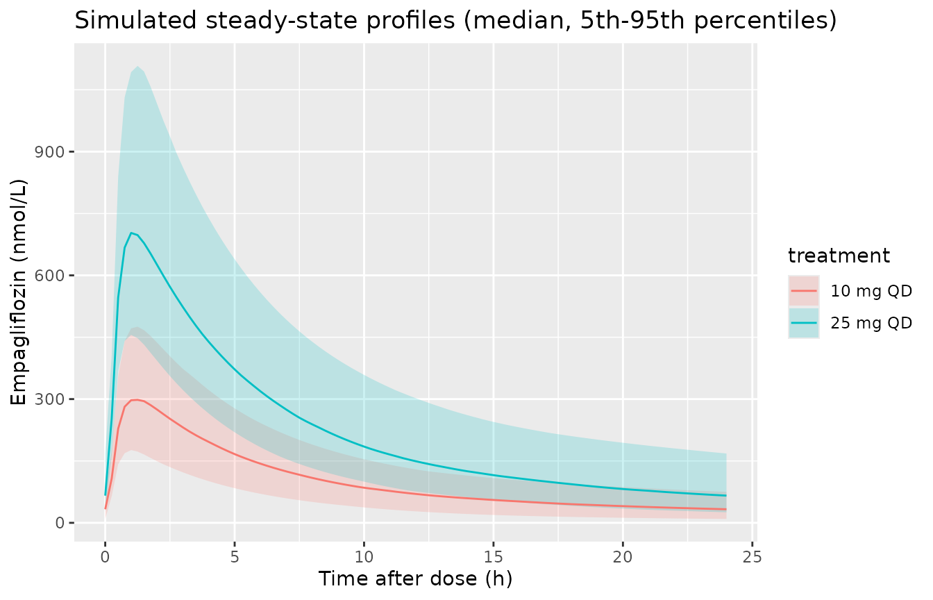
Steady-state AUC: closed-form check and Figure 3
At steady state AUC over the dosing interval equals dose / CL/F exactly, which is how the authors derived AUCss. The trapezoidal AUC of the simulated profiles must reproduce it; both sides use the same subject parameters, so the only difference is the 0.25-h trapezoid and integrator error.
mw <- 450.91
auc_ss <- sim_pk |>
  filter(time >= t_last) |>
  group_by(id, treatment, dose) |>
  summarise(
    auc_trap = sum(diff(time) * (head(Cc, -1) + tail(Cc, -1)) / 2),
    cl = cl[1],
    .groups = "drop"
  ) |>
  mutate(auc_cf = dose * 1e6 / mw / cl)
stopifnot(all(abs(auc_ss$auc_trap / auc_ss$auc_cf - 1) < 0.01))

auc_ss |>
  group_by(treatment) |>
  summarise(median_AUCss = median(auc_cf), q25 = quantile(auc_cf, 0.25),
            q75 = quantile(auc_cf, 0.75), median_CL = median(cl), .groups = "drop") |>
knitr::kable(digits = c(0, 0, 0, 0, 2))| treatment | median_AUCss | q25 | q75 | median_CL |
|---|---|---|---|---|
| 10 mg QD | 2469 | 1818 | 3183 | 8.98 |
| 25 mg QD | 5426 | 4312 | 7161 | 10.22 |
Figure 3 of the paper shows simulated paediatric AUCss for 10 mg once daily with a median of about 2300 nmolh/L and an interquartile range of about 1800-2950 nmolh/L (digitised by the maintainers).
ggplot(filter(auc_ss, dose == 10), aes(x = "Paediatric (10 mg)", y = auc_cf)) +
  geom_boxplot(fill = "#5ec8cc") +
  geom_hline(yintercept = 2300, linetype = "dashed") +
  labs(x = NULL, y = "Empagliflozin AUCss (nmol*h/L)",
       title = "Replicates Figure 3 of Rascher 2025 (paediatric arm)",
       caption = "Dashed line: published median, digitised (about 2300 nmol*h/L).")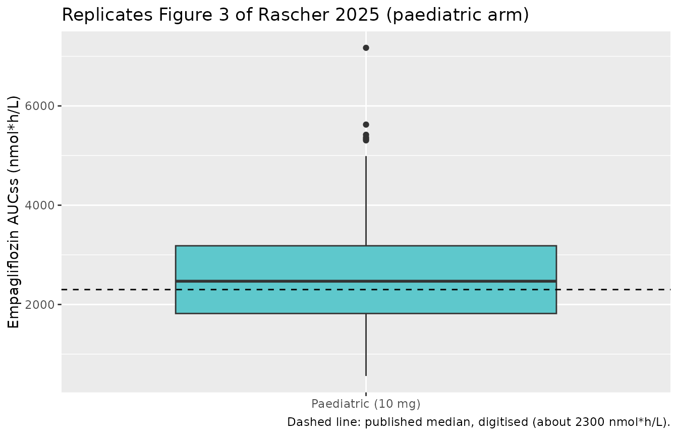
NCA with PKNCA
conc_df <- sim_pk |>
  filter(!is.na(Cc)) |>
  select(id, time, Cc, treatment)
dose_df <- ev_pk |>
  filter(evid == 1) |>
  select(id, time, amt, treatment)

conc_obj <- PKNCA::PKNCAconc(conc_df, Cc ~ time | treatment + id,
                             concu = "nmol/L", timeu = "h")
dose_obj <- PKNCA::PKNCAdose(dose_df, amt ~ time | treatment + id, doseu = "mg")
intervals <- data.frame(start = t_last, end = t_last + tau,
                        cmax = TRUE, tmax = TRUE, cmin = TRUE, auclast = TRUE)
nca_res <- PKNCA::pk.nca(PKNCA::PKNCAdata(conc_obj, dose_obj, intervals = intervals))

reference <- data.frame(treatment = "10 mg QD", auclast = 2300)
nlmixr2lib::ncaComparisonTable(
  nca_res, reference, by = "treatment",
  params = c("cmax", "tmax", "cmin", "auclast"),
  units = c(cmax = "nmol/L", tmax = "h", cmin = "nmol/L", auclast = "nmol*h/L"),
  label_first_column = "NCA parameter"
) |>
knitr::kable()| NCA parameter | treatment | Reference | Simulated | % diff |
|---|---|---|---|---|
| AUClast (nmol*h/L) | 10 mg QD | 2300 | 2470 | +7.3% |
The paper reports no NCA table; the only published reference is the digitised Figure 3 median AUCss at 10 mg (shown as AUC over the dosing interval at steady state).
The full simulated steady-state NCA summary by dose:
| Interval Start | Interval End | treatment | N | AUClast (h*nmol/L) | Cmax (nmol/L) | Cmin (nmol/L) | Tmax (h) |
|---|---|---|---|---|---|---|---|
| 216 | 240 | 10 mg QD | 200 | 2370 [43.0] | 296 [31.7] | 30.6 [71.4] | 1.25 [0.750, 1.50] |
| 216 | 240 | 25 mg QD | 200 | 5480 [38.4] | 705 [28.5] | 67.1 [63.2] | 1.00 [0.750, 1.50] |
HbA1c exposure-response
Typical-value time course (Figure S3)
A typical paediatric patient with eGFR 125 mL/min/1.73 m^2 (truncated to 120 in the model), observed baseline HbA1c equal to the model baseline, and AUCss 2300 nmol*h/L (the Figure 3 median at 10 mg), simulated on placebo and on empagliflozin with and without background insulin. Time 0 is the baseline HbA1c observation.
mod_pd_typ <- rxode2::zeroRe(mod_pd)
#> Warning: some etas defaulted to non-mu referenced, possible parsing error: etadp_slope
#> as a work-around try putting the mu-referenced expression on a simple line
wk <- c(0, 4, 12, 26)
typ <- tidyr::crossing(insulin = 0:1, auc = c(0, 2300)) |>
  mutate(id = row_number())
ev_typ <- typ |>
  tidyr::crossing(time = seq(0, 26 * 168, by = 24)) |>
  mutate(evid = 0L, cmt = "Hba1c", CONMED_INSULIN = insulin, AUC_EMPA = auc,
         HBA1C = 7.35 * 1.15^insulin, CRCL = 125)
sim_typ <- rxode2::rxSolve(mod_pd_typ, events = ev_typ, returnType = "data.frame",
                           keep = c("insulin", "auc"))
#> ℹ omega/sigma items treated as zero: 'etalrbase', 'etadp_slope'
#> Warning: multi-subject simulation without without 'omega'
pbo_adj_typ <- sim_typ |>
  select(time, insulin, auc, Hba1c) |>
  tidyr::pivot_wider(names_from = auc, values_from = Hba1c, names_prefix = "auc_") |>
  mutate(pbo_adj = auc_2300 - auc_0, week = time / 168,
         group = ifelse(insulin == 1, "Baseline insulin", "No baseline insulin"))

ggplot(pbo_adj_typ, aes(week, pbo_adj)) +
  geom_line() +
  facet_wrap(~group) +
  labs(x = "Time (week)", y = "Placebo-adjusted HbA1c change (%)",
       title = "Typical paediatric patient, 10 mg (compare Figure S3, median line)")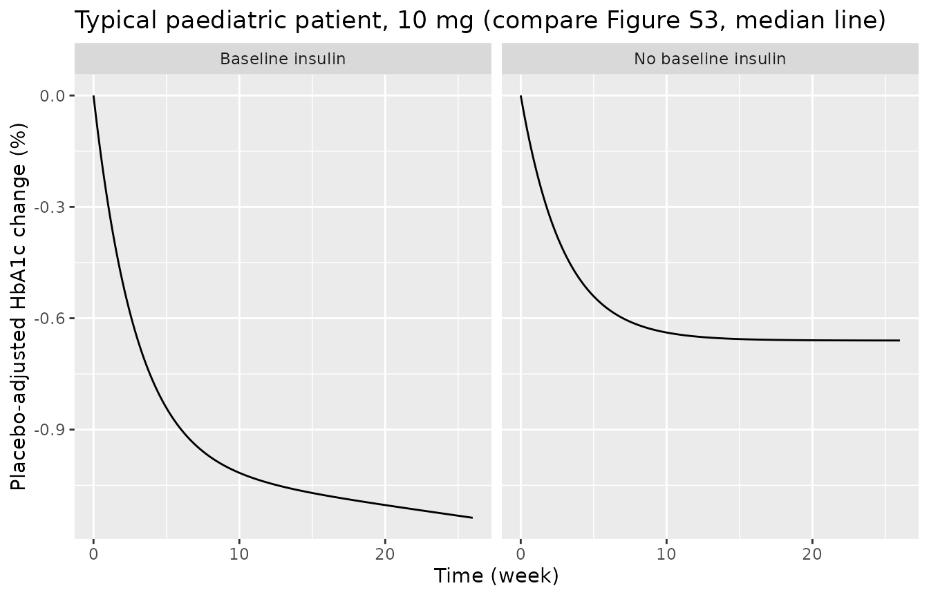
wk26 <- filter(pbo_adj_typ, time == 26 * 168) |> select(group, pbo_adj)
knitr::kable(wk26, digits = 3)| group | pbo_adj |
|---|---|
| No baseline insulin | -0.660 |
| Baseline insulin | -1.137 |
Figure S3 / Figure 4 show paediatric median placebo-adjusted changes at week 26 of about -1.07% with baseline insulin and -0.70% without (digitised). The typical patient reproduces both within 10%:
ref_fig4 <- c(`Baseline insulin` = -1.07, `No baseline insulin` = -0.70)
rel <- wk26$pbo_adj / ref_fig4[wk26$group] - 1
stopifnot(all(abs(rel) < 0.10))
The placebo course of the insulin group carries the disease progression: the typical HbA1c rises by about 1.1 percentage points over 26 weeks, matching the prediction-corrected placebo change from baseline of about +1% at 4400 h in Figure 2B.
sim_typ |>
  filter(auc == 0, time %in% (wk * 168)) |>
  group_by(insulin) |>
  reframe(week = time / 168, cfb = Hba1c - Hba1c[1]) |>
  tidyr::pivot_wider(names_from = week, values_from = cfb, names_prefix = "week_") |>
knitr::kable(digits = 3)| insulin | week_0 | week_4 | week_12 | week_26 |
|---|---|---|---|---|
| 0 | 0 | 0.000 | 0.000 | 0.000 |
| 1 | 0 | 0.085 | 0.424 | 1.073 |
Placebo-adjusted change in a virtual cohort (Figure 4)
Figure 4 shows the distribution of each simulated patient’s placebo-adjusted change. Each virtual patient is solved twice – on placebo and on 10 mg – with the same random effects, by drawing the BASE / PROG etas outside rxode2 and passing them as parameters to the zero-random-effect model. Each patient’s AUCss is dose / CL/F from the 10-mg PK cohort above, and the observed baseline HbA1c covariate is set to the patient’s model baseline.
om <- mod_pd$omega
set.seed(26)
pd_cohort <- auc_ss |>
  filter(dose == 10) |>
  select(id, auc = auc_cf) |>
  left_join(select(cohort, id, CRCL), by = "id") |>
  slice(rep(seq_len(n()), 2)) |>
  mutate(insulin = rep(0:1, each = n_arm), pid = row_number())
# Base-R draws (set.seed) keep the cohort identical across rxode2 builds.
etas <- matrix(rnorm(2 * nrow(pd_cohort)), ncol = 2) %*% chol(unclass(om)[1:2, 1:2])
pd_cohort$etalrbase <- etas[, 1]
pd_cohort$etadp_slope <- etas[, 2]
pd_cohort$HBA1C <- 7.35 * 1.15^pd_cohort$insulin * exp(pd_cohort$etalrbase)

paired <- bind_rows(
  mutate(pd_cohort, arm = "placebo", AUC_EMPA = 0),
  mutate(pd_cohort, arm = "empagliflozin", AUC_EMPA = auc)
) |>
  mutate(sid = row_number())
ev_pd <- paired |>
  tidyr::crossing(time = wk * 168) |>
  transmute(id = sid, time, evid = 0L, cmt = "Hba1c", CONMED_INSULIN = insulin,
            AUC_EMPA, HBA1C, CRCL) |>
  arrange(id, time)
# `params` rows are matched to subjects in order, so both frames are sorted by id.
prm <- transmute(paired, id = sid, etalrbase, etadp_slope) |>
  arrange(id)
sim_pd <- rxode2::rxSolve(mod_pd_typ, events = ev_pd, params = prm,
                          returnType = "data.frame")
#> Warning: multi-subject simulation without without 'omega'
sim_pd$id <- as.integer(as.character(sim_pd$id))
sim_pd <- sim_pd |>
  left_join(select(paired, id = sid, pid, arm, insulin, HBA1C), by = "id")
# Each subject must carry its own eta: the solved baseline equals the
# baseline built from that subject's eta draw.
chk_base <- filter(sim_pd, time == 0)
stopifnot(max(abs(chk_base$rbase / chk_base$HBA1C - 1)) < 1e-8)
#> Warning in max(abs(chk_base$rbase/chk_base$HBA1C - 1)): no non-missing
#> arguments to max; returning -Inf

pbo_adj <- sim_pd |>
  select(pid, insulin, arm, time, Hba1c) |>
  tidyr::pivot_wider(names_from = arm, values_from = Hba1c) |>
  mutate(pbo_adj = empagliflozin - placebo,
         group = ifelse(insulin == 1, "Baseline insulin", "No baseline insulin"))

wk26_cohort <- pbo_adj |>
  filter(time == 26 * 168) |>
  group_by(group) |>
  summarise(median = median(pbo_adj), q25 = quantile(pbo_adj, 0.25),
            q75 = quantile(pbo_adj, 0.75), .groups = "drop")
knitr::kable(wk26_cohort, digits = 3)| group | median | q25 | q75 |
|---|---|---|---|
| Baseline insulin | -1.101 | -1.469 | -0.770 |
| No baseline insulin | -0.583 | -0.850 | -0.438 |
ggplot(filter(pbo_adj, time == 26 * 168), aes(group, pbo_adj, colour = group)) +
  geom_boxplot() +
  geom_point(data = data.frame(group = names(ref_fig4), pbo_adj = ref_fig4),
             shape = 4, size = 4, colour = "black") +
  labs(x = NULL, y = "Placebo-adjusted HbA1c change from baseline (%)",
       title = "Replicates Figure 4 of Rascher 2025 (paediatric, 10 mg, week 26)",
       caption = "Crosses: published medians, digitised.") +
  theme(legend.position = "none")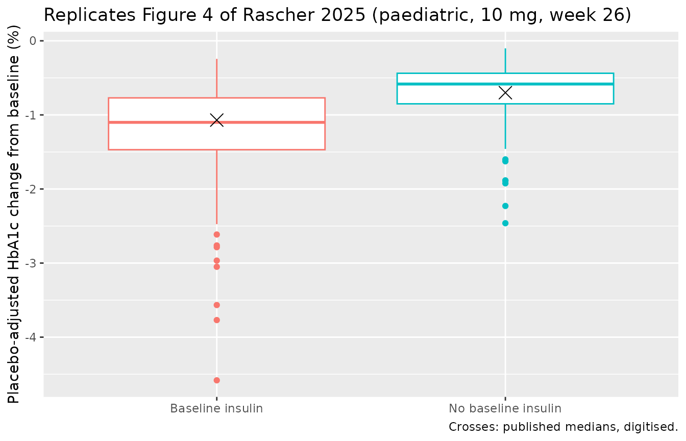
# Envelope gate: the structural check is the typical-value one above.
stopifnot(all(abs(wk26_cohort$median / ref_fig4[wk26_cohort$group] - 1) < 0.25))
The digitised interquartile ranges in Figure 4 are about -1.55 to -0.73 (insulin) and -1.02 to -0.47 (no insulin). The virtual-cohort medians sit below the published ones, by about 15% without insulin. Baseline HbA1c is not tabulated in the paper, so the cohort centres it on the model baseline; the published simulation presumably used the observed DINAMO baselines. Because the drug effect scales roughly with baseline HbA1c to the power 3 (2.04 in Imax plus 1 through the turnover), a baseline 0.25 percentage points higher would close the gap. The typical-value comparison above is the structural check; this one is an envelope. The abstract quotes a paediatric placebo-adjusted decrease of -0.699% at week 26 without stating the insulin mix; it matches the no-insulin group.
Assumptions and deviations
- Reference sex. The Results state that typical values refer to “a non-Black, non-Asian, female” subject, but the supplement equation adds the sex effect when FEMALE = 1 and Table 3 labels 1.19 as the “Sex = Female effect”. The model follows the equation: the reference is male and females have 1.19-fold CL/F.
- Outlier residual error. The PK residual error has a third, additive term (SD 353 nmol/L, Table 3 Sigma 3,3) applied only to observations the authors flagged as outliers. That flag is a property of the fitted data set, so the model carries only the non-outlier proportional + additive error.
- Imax covariate form. The supplement prints IMAX_eGFR = (eGFR/90) x theta and IMAX_HbA1c = (HbA1c/7.9) x theta, but its text describes both as normalised covariates “with an estimated exponent”. The power form is used; it reproduces the Figure 4 medians, whereas the multiplicative reading would roughly double the drug effect.
-
PROG random effect. The supplement adds eta3/100000
to the progression rate, so the eta is additive and present also in
patients without insulin. Table 4 prints its magnitude as “CV 7.35%”;
the variance is taken as log(1 + 0.0735^2) = 0.005388 by the table
footnote (0.0735^2 = 0.005402 differs by 0.3%). The eta is named
etadp_slopewithout the log prefix ofldp_slopebecause it does not act on the log scale. - PROG-BASE off-diagonal. Table 4 labels 0.00112 “Covariance on PROG-BASE” under a “Corr” heading; it is used as the covariance (correlation 0.095). Read as a correlation it would be 1.3e-05; either way the two random effects are nearly independent.
- Disease progression. dkin/dt = PROG with kin(0) = BASE x kout is integrated in closed form, kin = BASE x kout + PROG x t, so simulations must start at the baseline HbA1c observation (t = 0).
- Time units. The model runs in hours; kout is stored in its Table 4 unit (1/day) and divided by 24. Figure 2’s hour axis and the %/h/h unit of PROG confirm hours.
- Molecular weight. Concentrations and AUC are in nmol/L and nmol*h/L; the paper does not print the molecular weight. 450.91 g/mol (C23H27ClO7) is used, as in the other empagliflozin models in this package.
- Virtual cohorts. Covariate distributions are reconstructed from the summary statistics of Tables S1 and S2; baseline HbA1c is not tabulated in the paper and is set to each patient’s model baseline. The paper’s own simulation cohorts are not described in detail, so the comparisons with Figures 3 and 4 use the median and are gated at 15% (Figure 3) and 25% (Figure 4 cohort); the deterministic typical-value check against Figure 4 is gated at 10%.
- Errata. No erratum was found (literature check 2026-11-05).