51Cr-EDTA and 99mTc-DTPA GFR tracers (Gracia 2025)
Source:vignettes/articles/Gracia_2025_cr51edta_tc99mdtpa.Rmd
Gracia_2025_cr51edta_tc99mdtpa.RmdModel and source
#> ℹ parameter labels from comments will be replaced by 'label()'
#> Warning: some etas defaulted to non-mu referenced, possible parsing error: etaiov_cl_1, etaiov_cl_2, etaiov_cl_3, etaiov_cl_4, etaiov_cl_5
#> as a work-around try putting the mu-referenced expression on a simple line
Citation: Gracia M, Ankaoua V, Alonso M, Pasquet M, Chatelut E. A population pharmacokinetic approach to compare (51)Cr-EDTA and (99 m)Tc-DTPA clearances in measuring renal glomerular filtration rate in oncopediatrics. Pediatr Nephrol. 2025;40(10):3163-3168. doi:10.1007/s00467-025-06828-9.
Description: One-compartment IV-bolus population PK model fitted simultaneously to 51Cr-EDTA and 99mTc-DTPA plasma concentrations in 59 oncopediatric children (40 51Cr-EDTA / 19 99mTc-DTPA) receiving cisplatin and/or ifosfamide (Gracia 2025). Clearance is the measured glomerular filtration rate and follows the CYSPED power equation on serum creatinine, plasma cystatin C and body weight; volume is proportional to body weight. A binary per-record tracer indicator (TRACER_TC99M_DTPA; the paper’s MES covariate) enters both CL and V multiplicatively as (1 - theta * TRACER_TC99M_DTPA) and carries the paper’s estimand, the inter-tracer bias of -0.9% (95% CI +/- 11.4%) on clearance. Inter-occasion variability is carried on CL, and the proportional residual error is tracer-specific.
Article: https://doi.org/10.1007/s00467-025-06828-9 (Pediatric Nephrology 2025;40:3163-3168; PMC12401762, open access)
Gracia 2025 asks whether the two reference radioisotopic methods for
measuring glomerular filtration rate in children – chromium-51 EDTA and
technetium-99m DTPA – give the same answer. In adults the question has
been settled by giving both tracers to the same volunteer
simultaneously, but that design is not ethically available in children.
The authors instead fit a single population PK model jointly to
both tracers’ plasma concentrations, with a binary per-record
tracer indicator (MES in the paper,
TRACER_TC99M_DTPA here) carried on both clearance and
volume. The coefficient on that indicator is the inter-tracer
bias, and the covariate model absorbs the demographic differences
between the two non-overlapping patient groups.
Clearance in this model is the measured GFR, so the packaged model doubles as an implementation of the CYSPED paediatric GFR equation re-estimated on 59 children.
Population
| Field | Value |
|---|---|
| species | human |
| n_subjects | 59 |
| n_studies | 2 |
| age_range | 1.4-17.8 years (51Cr-EDTA group); 2.0-16.3 years (99mTc-DTPA group) |
| age_mean | 10.6 years (51Cr-EDTA group); 10.1 years (99mTc-DTPA group) |
| weight_range | 9.07-72.0 kg (51Cr-EDTA group); 10.0-91.8 kg (99mTc-DTPA group) |
| weight_mean | 34.3 kg (51Cr-EDTA group); 42.9 kg (99mTc-DTPA group) |
| sex_female_pct | 55.9 |
| disease_state | Pediatric malignancy (osteosarcoma 33, neuroblastoma 9, germinal tumor 7, rhabdomyosarcoma 3, other 7) treated with cisplatin and/or ifosfamide and requiring GFR monitoring for chemotherapy nephrotoxicity |
| dose_range | 2.072 MBq 51Cr-EDTA IV bolus; 6, 9 or 12 MBq 99mTc-DTPA IV bolus for body weight < 10 kg, 10-20 kg and > 20 kg respectively |
| regions | France (Toulouse University Hospital) |
| renal_function | Not restricted at inclusion; GFR monitored for nephrotoxicity of cisplatin and/or ifosfamide |
| notes | Baseline demographics from Gracia 2025 Table 1 (characteristics before the first GFR measurement). 40 children from the Cysped clinical trial (NCT02822404, 51Cr-EDTA, February 2012 to September 2015) and 19 from the CysPedVal analysis (RnIPH 2020-101, 99mTc-DTPA, December 2020 to June 2022). Inclusion criteria: age 0-18 years and body weight over 4 kg. Sex 26 male / 33 female overall (18/22 and 8/11 by group). Each tracer was given as an IV bolus twice per patient (before chemotherapy and at end of treatment) with four blood samples drawn from the contralateral arm at 90, 110, 130 and 150 min. Between one and five (median three) GFR measurements per patient. No patient received both tracers. |
Fifty-nine oncopediatric children contributed data: 40 from the Cysped trial (NCT02822404, 51Cr-EDTA, February 2012 to September 2015) and 19 from the CysPedVal analysis (RnIPH 2020-101, 99mTc-DTPA, December 2020 to June 2022). All were treated with cisplatin and/or ifosfamide and required GFR monitoring for chemotherapy nephrotoxicity. Baseline characteristics are Gracia 2025 Table 1; the two groups differed significantly in body weight (34.3 vs 42.9 kg, p = 1e-4) and plasma cystatin C (0.76 vs 0.82 mg/L, p = 8e-6) but not in age, sex, height or serum creatinine. No patient received both tracers, so tracer identity is perfectly confounded with source study in the observed data; the covariate model is what makes the two groups comparable.
Each tracer was given as an IV bolus twice per patient (before chemotherapy and at the end of treatment), with four blood samples drawn from the contralateral arm at 90, 110, 130 and 150 min. Between one and five (median three) GFR measurements were taken per patient. The dose was 2.072 MBq for 51Cr-EDTA, and 6, 9 or 12 MBq for 99mTc-DTPA at body weights below 10 kg, 10-20 kg and above 20 kg respectively.
Source trace
Every ini() entry in
inst/modeldb/specificDrugs/Gracia_2025_cr51edta_tc99mdtpa.R
carries an in-file comment naming its source location. They are
collected here for review.
| Equation / parameter | Value | Source location |
|---|---|---|
TVCL = theta1 * (Scr/42.25)^theta3 * (PcysC/0.7738)^theta4 * (BW/35.70)^theta5 * (1 - theta6 * MES) |
n/a | Table 2, “Clearance (CL) (mL/min)” row |
TVV = theta7 * BW * (1 - theta8 * MES) |
n/a | Table 2, “Volume of distribution (V) (mL)” row |
lcl (theta1) |
80.8 mL/min (+/- 3.1) | Table 2 |
e_creat_cl (theta3) |
-0.568 (+/- 0.156) | Table 2 |
e_cysc_cl (theta4) |
-0.295 (+/- 0.168) | Table 2 |
e_wt_cl (theta5) |
+1.06 (+/- 0.145) | Table 2 |
e_tracer_tc99m_dtpa_cl (theta6) |
-0.009 (+/- 0.114) | Table 2; restated in Results and in Table 3 row 1 |
lvc (theta7) |
256 mL/kg (+/- 20) | Table 2 |
e_tracer_tc99m_dtpa_vc (theta8) |
+0.017 (+/- 0.143) | Table 2; restated in Results |
etalcl |
11% CV -> variance log(0.11^2 + 1) | Table 2, “Interindividual variability (CV%)” under the CL block; Table 3 row 1 |
etalvc |
20.9% CV -> variance log(0.209^2 + 1) | Table 2, “Interindividual variability (CV%)” under the V block |
etaiov_cl_1 .. etaiov_cl_5
|
14.5% CV -> variance log(0.145^2 + 1) | Table 2, “Interoccasion variability (CV%)”; Methods “Interoccasion variability of CL was included” |
propSd_cr51edta |
4.99% CV | Table 2, “51Cr-EDTA plasma concentrations” |
propSd_tc99mdtpa |
7.18% CV | Table 2, “99mTc-DTPA plasma concentrations” |
| Centering constants 42.25 umol/L, 0.7738 mg/L, 35.70 kg | n/a | Table 2 CL equation as printed |
| One-compartment structure, IV bolus, FOCEI | n/a | Methods, “Pharmacokinetic analysis” |
| Dose amounts and sampling times | n/a | Methods, “Patients and data” |
| Number of occasions (1 to 5 per patient) | n/a | Methods, “Patients and data” |
Virtual cohort
Individual patient data are not public (Gracia 2025 Data availability: “Data are available on request from the corresponding author”), so the checks below use virtual children whose covariate marginals follow Gracia 2025 Table 1.
The design is deliberately paired: every virtual child is simulated twice, once with each tracer, holding body weight, serum creatinine, cystatin C and the random effects fixed. That is the simultaneous-administration design the paper calls the gold standard and could not run in children, so it isolates the tracer effect exactly.
set.seed(20250529)
n_child <- 200  # per tracer arm (cap: 200/arm)

# Table 2 parameters, read back from the packaged model so this vignette can
# never drift from inst/modeldb/.
p <- list(
  cl_ref   = exp(theta[["lcl"]]),
  v_per_kg = exp(theta[["lvc"]]),
  e_creat  = theta[["e_creat_cl"]],
  e_cysc   = theta[["e_cysc_cl"]],
  e_wt     = theta[["e_wt_cl"]],
  e_tr_cl  = theta[["e_tracer_tc99m_dtpa_cl"]],
  e_tr_v   = theta[["e_tracer_tc99m_dtpa_vc"]]
)
# Centering constants as printed in the Table 2 equation.
ref <- list(creat = 42.25, cysc = 0.7738, wt = 35.70)

# Independent re-implementation of the Table 2 typical-value equations. Used
# below as a cross-check on the packaged model() block.
tvcl <- function(CREAT, CYSC, WT, MES) {
  p$cl_ref * (CREAT / ref$creat)^p$e_creat * (CYSC / ref$cysc)^p$e_cysc *
    (WT / ref$wt)^p$e_wt * (1 - p$e_tr_cl * MES)
}
tvv <- function(WT, MES) p$v_per_kg * WT * (1 - p$e_tr_v * MES)

# 99mTc-DTPA bolus, Methods "Patients and data": 6 / 9 / 12 MBq for body
# weight < 10 / 10-20 / > 20 kg. 51Cr-EDTA is 2.072 MBq at every weight.
dtpa_dose <- function(WT) ifelse(WT < 10, 6, ifelse(WT <= 20, 9, 12))
edta_dose <- function(WT) rep(2.072, length(WT))

# Truncated log-normal draws matched to the Table 1 pooled marginals.
rtrunc_lnorm <- function(n, med, cv, lo, hi) {
  sdlog <- sqrt(log(cv^2 + 1))
  x <- rlnorm(n, log(med), sdlog)
  pmin(pmax(x, lo), hi)
}

subjects <- tibble::tibble(
  child = seq_len(n_child),
  # Table 1 pooled body weight: means 34.3 (EDTA) and 42.9 kg (DTPA),
  # observed range 9.07-91.8 kg.
  WT    = rtrunc_lnorm(n_child, med = 33, cv = 0.50, lo = 9.07, hi = 91.8),
  # Table 1 serum creatinine: mean 42 umol/L both groups, range 8-102.
  CREAT = rtrunc_lnorm(n_child, med = 40, cv = 0.40, lo = 8, hi = 102),
  # Table 1 plasma cystatin C: means 0.76 / 0.82 mg/L, range 0.26-1.36.
  CYSC  = rtrunc_lnorm(n_child, med = 0.77, cv = 0.25, lo = 0.26, hi = 1.36)
)

# The study's four sampling times (Methods, "Patients and data").
obs_times <- c(90, 110, 130, 150)

# Observation grid for NCA. Terminal half-life runs about 55-120 min across the
# cohort's covariate range, so 720 min is 6-13 half-lives -- long enough for a
# small AUC extrapolation without decaying into solver noise. PKNCA's default
# lin-up/log-down trapezoid is exact for a mono-exponential decay, so a 5-min
# grid is as accurate as a much finer one and far cheaper to solve.
grid_nca <- seq(0, 720, by = 5)

# Sparse grid reproducing the study's own design, used for the stochastic runs.
grid_obs <- c(0, obs_times)

make_arm <- function(subj, tracer, id_offset, grid = grid_nca) {
  mes  <- as.integer(tracer == "99mTc-DTPA")
  dose <- if (mes == 1L) dtpa_dose(subj$WT) else edta_dose(subj$WT)
  base <- subj |>
    dplyr::mutate(
      id = id_offset + child,
      TRACER_TC99M_DTPA = mes,
      OCC = 1L,
      tracer = tracer,
      dose = dose
    )
  dosing <- base |>
    dplyr::mutate(time = 0, amt = dose, evid = 1L, cmt = "central")
  obs <- base |>
    tidyr::crossing(time = grid) |>
    dplyr::mutate(amt = NA_real_, evid = 0L, cmt = "central")
  dplyr::bind_rows(dosing, obs) |>
    dplyr::arrange(id, time, dplyr::desc(evid)) |>
    dplyr::select(id, time, amt, evid, cmt, WT, CREAT, CYSC,
                  TRACER_TC99M_DTPA, OCC, tracer, dose)
}

# Rich-grid event table for the typical-value / NCA work.
events <- dplyr::bind_rows(
  make_arm(subjects, "51Cr-EDTA",  id_offset = 0L),
  make_arm(subjects, "99mTc-DTPA", id_offset = as.integer(n_child))
)

# Same children and same IDs, sampled only at the study's four times, for the
# stochastic runs (Figure 1 and the residual-error check).
events_obs <- dplyr::bind_rows(
  make_arm(subjects, "51Cr-EDTA",  id_offset = 0L,                  grid = grid_obs),
  make_arm(subjects, "99mTc-DTPA", id_offset = as.integer(n_child), grid = grid_obs)
)

# Disjoint IDs across arms (rxSolve silently merges duplicated ids).
for (ev_tbl in list(events, events_obs)) {
  stopifnot(!anyDuplicated(unique(ev_tbl[, c("id", "time", "evid")])))
  stopifnot(length(intersect(
    unique(ev_tbl$id[ev_tbl$tracer == "51Cr-EDTA"]),
    unique(ev_tbl$id[ev_tbl$tracer == "99mTc-DTPA"])
  )) == 0L)
}
Simulation
The typical-value simulation (zeroRe()) is used for the
structural checks and the NCA comparison; the stochastic simulation is
used to reproduce Figure 1 and to recover the published variance
components.
omega is passed explicitly on every
solve. rxode2 caches the previous solve’s omega against the
compiled model, so a zeroRe() model can silently re-sample
etas and a population model can silently lose its IIV;
omega = NA and omega = ui$omega pin each
direction.
# Tight solver tolerances: this profile feeds the per-subject NCA identities
# (Dose / AUC0-inf = CL, CL / lambda_z = V) that are asserted to 1e-8 below,
# and the default rtol of 1e-6 leaves ~1e-6 relative error in both.
sim_typ <- rxode2::rxSolve(
  rxode2::zeroRe(ui), events = events, omega = NA,
  keep = c("tracer", "dose"), returnType = "data.frame",
  rtol = 1e-10, atol = 1e-12
)
#> Warning: No sigma parameters in the model
#> Warning: some etas defaulted to non-mu referenced, possible parsing error: etaiov_cl_1, etaiov_cl_2, etaiov_cl_3, etaiov_cl_4, etaiov_cl_5
#> as a work-around try putting the mu-referenced expression on a simple line
#> Warning: multi-subject simulation without without 'omega'

# With the random effects zeroed, each subject must have exactly one CL and one
# V, and they must equal the independent re-implementation of Table 2 above.
chk <- sim_typ |>
  dplyr::filter(!is.na(Cc)) |>
  dplyr::group_by(id, tracer) |>
  dplyr::summarise(cl = dplyr::first(cl), vc = dplyr::first(vc),
                   n_cl = dplyr::n_distinct(round(cl, 10)),
                   n_vc = dplyr::n_distinct(round(vc, 10)), .groups = "drop") |>
  dplyr::left_join(
    events |> dplyr::distinct(id, WT, CREAT, CYSC, TRACER_TC99M_DTPA),
    by = "id"
  )
stopifnot(all(chk$n_cl == 1L), all(chk$n_vc == 1L))
stopifnot(isTRUE(all.equal(
  chk$cl, tvcl(chk$CREAT, chk$CYSC, chk$WT, chk$TRACER_TC99M_DTPA),
  tolerance = 1e-8
)))
stopifnot(isTRUE(all.equal(
  chk$vc, tvv(chk$WT, chk$TRACER_TC99M_DTPA), tolerance = 1e-8
)))
set.seed(6828)
sim_iiv <- rxode2::rxSolve(
  ui$simulationModel, events = events_obs, omega = ui$omega,
  keep = c("tracer", "dose"), returnType = "data.frame"
)
# Guard the reverse direction of the same rxode2 cache bug: the population run
# must actually vary between subjects.
stopifnot(dplyr::n_distinct(round(sim_iiv$cl, 8)) > 1L)
stopifnot(dplyr::n_distinct(round(sim_iiv$vc, 8)) > 1L)
# rxode2 returns Cc == ipredSim (no residual error); `sim` carries the
# proportional residual error. Pin the distinction so it cannot regress.
stopifnot(isTRUE(all.equal(sim_iiv$Cc, sim_iiv$ipredSim)))
stopifnot(!isTRUE(all.equal(sim_iiv$Cc, sim_iiv$sim)))
sim_iiv <- dplyr::rename(sim_iiv, Cc_assay = sim)
The inter-tracer bias (the paper’s primary result)
Gracia 2025 Abstract: “Analysis revealed a non-significant bias
(+/- 95% CI) of -0.9% +/- 11.4% between the two measurements (with
99mTc-DTPA clearance overestimated).” In the model that bias is
theta6 entering as (1 - theta6 * MES), so the
ratio of the 99mTc-DTPA clearance to the 51Cr-EDTA clearance in the same
child is 1 - theta6.
ratio_tab <- chk |>
  dplyr::select(id, tracer, cl, vc, WT, CREAT, CYSC) |>
  dplyr::mutate(child = ifelse(tracer == "51Cr-EDTA", id, id - n_child)) |>
  dplyr::select(-id) |>
  tidyr::pivot_wider(names_from = tracer, values_from = c(cl, vc)) |>
  dplyr::mutate(
    cl_ratio = `cl_99mTc-DTPA` / `cl_51Cr-EDTA`,
    v_ratio  = `vc_99mTc-DTPA` / `vc_51Cr-EDTA`
  )

# Every child must show exactly the published bias, on both CL and V.
stopifnot(isTRUE(all.equal(ratio_tab$cl_ratio,
                           rep(1 - p$e_tr_cl, nrow(ratio_tab)), tolerance = 1e-10)))
stopifnot(isTRUE(all.equal(ratio_tab$v_ratio,
                           rep(1 - p$e_tr_v, nrow(ratio_tab)), tolerance = 1e-10)))

bias_cl_pct <- 100 * (mean(ratio_tab$cl_ratio) - 1)
bias_v_pct  <- 100 * (mean(ratio_tab$v_ratio) - 1)
Across all 200 virtual children the model gives a +0.9% difference in clearance and a -1.7% difference in volume for 99mTc-DTPA relative to 51Cr-EDTA.
Mind the sign convention, which is easy to invert. The paper quotes
the bias as the coefficient
theta6 = -0.009 (“a non-significant bias of -0.9%”), but
the coefficient enters as (1 - theta6 * MES), so a
negative coefficient makes the 99mTc-DTPA clearance 0.9%
higher. That is exactly what the abstract’s
parenthetical says – “with 99mTc-DTPA clearance overestimated” – and it
is the direction Biggi, Fleming and McMeekin all reported in adults
(Discussion). The same inversion applies to volume: the published
coefficient theta8 is +0.017, so the 99mTc-DTPA volume is 1.7%
lower. Both 95% confidence intervals (+/- 0.114 on CL,
+/- 0.143 on V) span zero, which is the paper’s conclusion: the two
tracers are equivalent.
| Quantity | Published | Packaged |
|---|---|---|
| Bias coefficient theta6 (CL) | -0.009 (95% CI +/- 0.11) | -0.009 |
| Interindividual variability on CL (CV%) | 11.0 | 11.0 |
Replicate published figures
Figure 1 – individual predicted vs. observed plasma concentrations
Gracia 2025 Figure 1 plots individual predicted against observed
plasma concentrations for 51Cr-EDTA (1a) and 99mTc-DTPA (1b). Here the
individual prediction is Cc and the “observation” is
Cc_assay, i.e. Cc with the tracer-specific
proportional residual error applied, evaluated at the study’s four
sampling times.
fig1 <- sim_iiv |>
  dplyr::filter(!is.na(Cc), time %in% obs_times)

ggplot(fig1, aes(Cc, Cc_assay)) +
  geom_point(alpha = 0.25, size = 0.7) +
  geom_abline(slope = 1, intercept = 0, colour = "red") +
  facet_wrap(~tracer, scales = "free") +
  labs(
    x = "Individual predicted concentration (MBq/mL)",
    y = "Observed concentration (MBq/mL)",
    title = "Figure 1 -- individual predicted vs. observed",
    caption = "Replicates Figure 1a/1b of Gracia 2025 (samples at 90, 110, 130 and 150 min)."
  )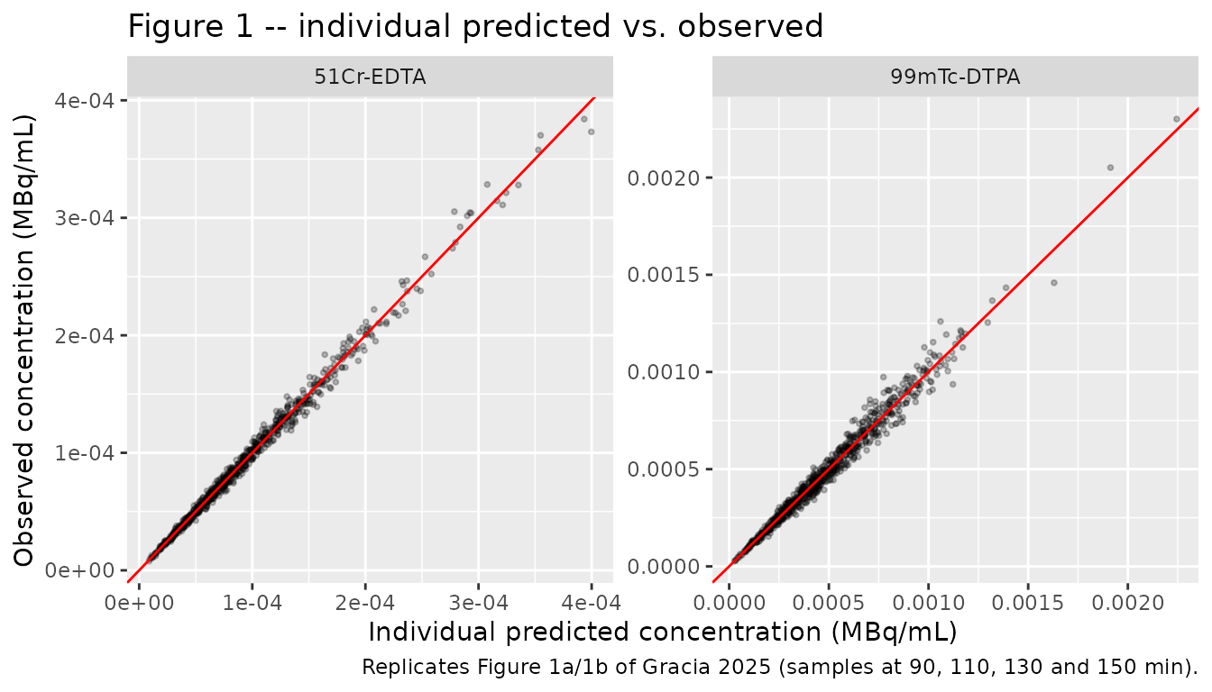
The scatter around the identity line is the tracer-specific residual error, and it should reproduce the two published magnitudes.
ruv <- fig1 |>
  dplyr::group_by(tracer) |>
  dplyr::summarise(cv_pct = 100 * sd(Cc_assay / Cc - 1), n = dplyr::n(),
                   .groups = "drop") |>
  dplyr::mutate(published_pct = ifelse(tracer == "51Cr-EDTA",
                                       100 * theta[["propSd_cr51edta"]],
                                       100 * theta[["propSd_tc99mdtpa"]]))
ruv |>
  dplyr::rename("Tracer" = tracer, "Simulated residual CV (%)" = cv_pct,
                "n samples" = n, "Published residual CV (%)" = published_pct) |>
knitr::kable(digits = 2, caption = "Residual error recovered from the simulation vs. Gracia 2025 Table 2.")| Tracer | Simulated residual CV (%) | n samples | Published residual CV (%) |
|---|---|---|---|
| 51Cr-EDTA | 4.80 | 800 | 4.99 |
| 99mTc-DTPA | 7.36 | 800 | 7.18 |
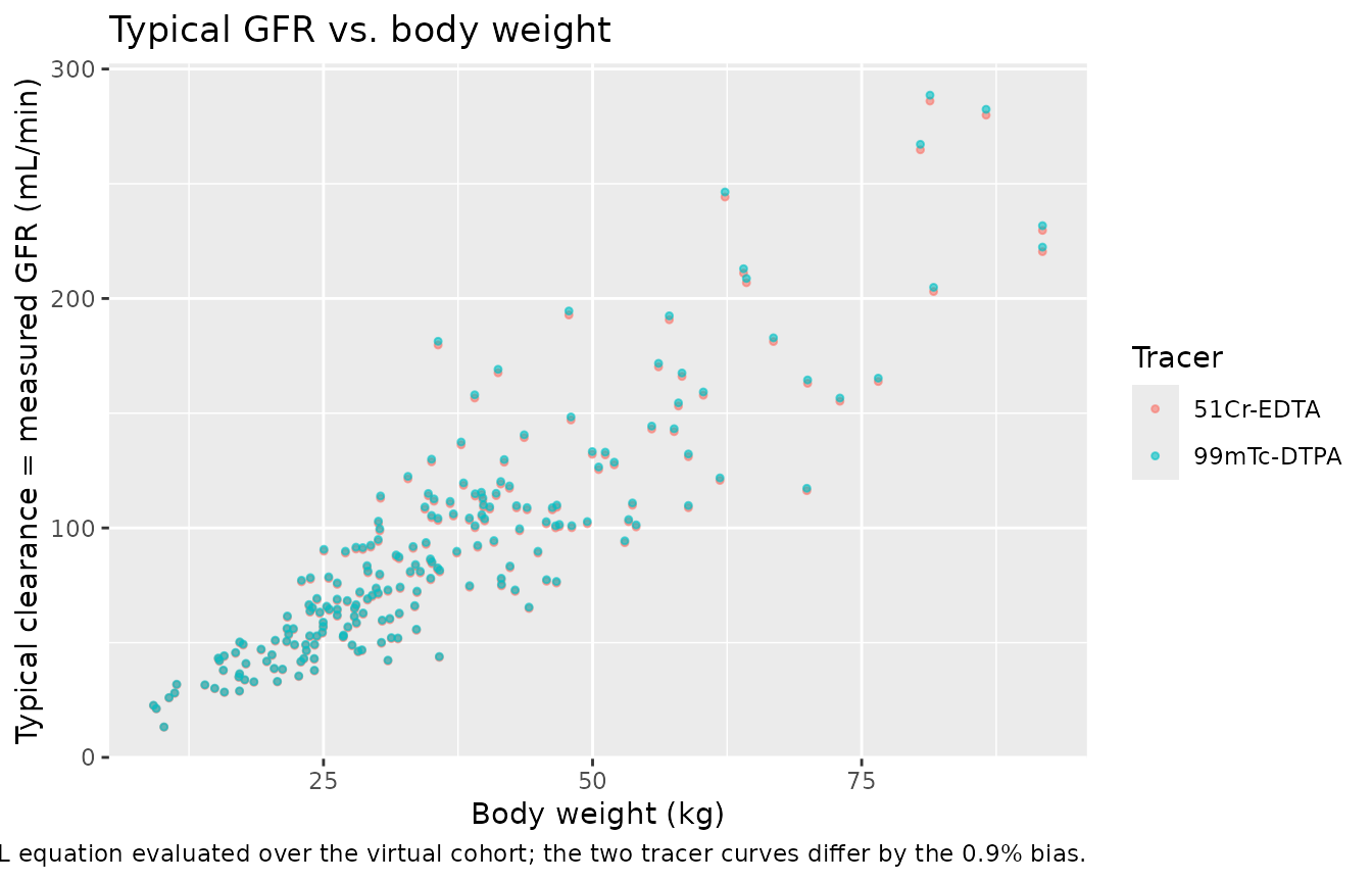
Typical GFR across the paediatric weight range
The CL equation is the CYSPED GFR equation, so the typical-value simulation is a direct rendering of it over the cohort’s covariate range.
chk |>
  ggplot(aes(WT, cl, colour = tracer)) +
  geom_point(alpha = 0.6, size = 0.9) +
  labs(
    x = "Body weight (kg)", y = "Typical clearance = measured GFR (mL/min)",
    colour = "Tracer",
    title = "Typical GFR vs. body weight",
    caption = "Table 2 CL equation evaluated over the virtual cohort; the two tracer curves differ by the 0.9% bias."
  )
PKNCA validation
For a one-compartment IV bolus, Dose / AUC0-inf recovers
clearance exactly and CL / lambda_z recovers the volume of
distribution. Both are computed with PKNCA from the typical-value
simulation and compared against the Table 2 equations, per subject.
sim_nca <- sim_typ |>
  dplyr::filter(!is.na(Cc)) |>
  dplyr::select(id, time, Cc, tracer)

# Guarantee a time = 0 row per (id, tracer). The rich grid already contains
# time = 0 (the post-bolus concentration), so .keep_all keeps the real value.
sim_nca <- dplyr::bind_rows(
  sim_nca,
  sim_nca |> dplyr::distinct(id, tracer) |> dplyr::mutate(time = 0, Cc = 0)
) |>
  dplyr::distinct(id, tracer, time, .keep_all = TRUE) |>
  dplyr::arrange(id, tracer, time)

stopifnot(all(sim_nca$Cc >= 0))

conc_obj <- PKNCA::PKNCAconc(sim_nca, Cc ~ time | tracer + id)

dose_df <- events |>
  dplyr::filter(evid == 1) |>
  dplyr::select(id, time, amt, tracer) |>
  dplyr::mutate(route = "intravascular", duration = 0)

dose_obj <- PKNCA::PKNCAdose(dose_df, amt ~ time | tracer + id)
#> Found column named route, using it for the attribute of the same name.
#> Found column named duration, using it for the attribute of the same name.

intervals <- data.frame(
  start = 0, end = Inf,
  cmax = TRUE, aucinf.obs = TRUE, half.life = TRUE,
  cl.obs = TRUE, vz.obs = TRUE
)

nca_res <- PKNCA::pk.nca(PKNCA::PKNCAdata(conc_obj, dose_obj, intervals = intervals))
nca_wide <- as.data.frame(nca_res) |>
  dplyr::select(tracer, id, PPTESTCD, PPORRES) |>
  tidyr::pivot_wider(names_from = PPTESTCD, values_from = PPORRES) |>
  dplyr::left_join(
    events |> dplyr::distinct(id, WT, CREAT, CYSC, TRACER_TC99M_DTPA),
    by = "id"
  ) |>
  dplyr::mutate(
    cl_model = tvcl(CREAT, CYSC, WT, TRACER_TC99M_DTPA),
    v_model  = tvv(WT, TRACER_TC99M_DTPA),
    cl_err   = cl.obs / cl_model - 1,
    v_err    = vz.obs / v_model - 1
  )

# Per-subject structural identities. The residual disagreement is pure
# trapezoidal / extrapolation error from the finite observation grid.
stopifnot(nrow(nca_wide) == 2L * n_child)
# PKNCA reproduces both to machine precision for this mono-exponential system,
# so the bound is tight enough to catch any structural regression.
stopifnot(max(abs(nca_wide$cl_err)) < 1e-8)
stopifnot(max(abs(nca_wide$v_err))  < 1e-8)

tibble::tibble(
  Identity = c("Dose / AUC0-inf vs. Table 2 CL equation",
               "CL / lambda_z vs. Table 2 V equation"),
  `Max |relative error|` = sprintf("%.3f%%", 100 * c(max(abs(nca_wide$cl_err)),
                                                     max(abs(nca_wide$v_err)))),
  `Subjects checked` = nrow(nca_wide)
) |>
knitr::kable(caption = "Per-subject NCA identities across both tracer arms.")| Identity | Max |relative error| | Subjects checked |
|---|---|---|
| Dose / AUC0-inf vs. Table 2 CL equation | 0.000% | 400 |
| CL / lambda_z vs. Table 2 V equation | 0.000% | 400 |
Comparison against published values
Gracia 2025 reports no NCA table, so the reference column below is
built from the Table 2 equations evaluated at the model’s own reference
covariate set (serum creatinine 42.25 umol/L, cystatin C 0.7738 mg/L,
body weight 35.70 kg) – the covariate set at which theta1
and theta7 are the typical values. A reference child is
simulated at exactly that covariate set for each tracer.
ref_subj <- tibble::tibble(child = 1L, WT = ref$wt, CREAT = ref$creat, CYSC = ref$cysc)
ref_events <- dplyr::bind_rows(
  make_arm(ref_subj, "51Cr-EDTA",  id_offset = 0L),
  make_arm(ref_subj, "99mTc-DTPA", id_offset = 1L)
)
ref_sim <- rxode2::rxSolve(
  rxode2::zeroRe(ui), events = ref_events, omega = NA,
  keep = c("tracer", "dose"), returnType = "data.frame"
)
#> Warning: No sigma parameters in the model
#> Warning: some etas defaulted to non-mu referenced, possible parsing error: etaiov_cl_1, etaiov_cl_2, etaiov_cl_3, etaiov_cl_4, etaiov_cl_5
#> as a work-around try putting the mu-referenced expression on a simple line
#> Warning: multi-subject simulation without without 'omega'

ref_nca_in <- ref_sim |>
  dplyr::filter(!is.na(Cc)) |>
  dplyr::select(id, time, Cc, tracer) |>
  dplyr::arrange(id, time)
ref_dose <- ref_events |>
  dplyr::filter(evid == 1) |>
  dplyr::select(id, time, amt, tracer) |>
  dplyr::mutate(route = "intravascular", duration = 0)

ref_res <- PKNCA::pk.nca(PKNCA::PKNCAdata(
  PKNCA::PKNCAconc(ref_nca_in, Cc ~ time | tracer + id),
  PKNCA::PKNCAdose(ref_dose, amt ~ time | tracer + id),
  intervals = intervals
))
#> Found column named route, using it for the attribute of the same name.
#> Found column named duration, using it for the attribute of the same name.
# Table 2 predictions for the reference child, computed from the packaged
# thetas rather than transcribed, so they cannot drift.
ref_dose_amt <- c(`51Cr-EDTA` = edta_dose(ref$wt), `99mTc-DTPA` = dtpa_dose(ref$wt))
published <- tibble::tibble(
  tracer     = c("51Cr-EDTA", "99mTc-DTPA"),
  mes        = c(0, 1)
) |>
  dplyr::mutate(
    cl.obs     = tvcl(ref$creat, ref$cysc, ref$wt, mes),
    vz.obs     = tvv(ref$wt, mes),
    half.life  = log(2) * vz.obs / cl.obs,
    cmax       = unname(ref_dose_amt[tracer]) / vz.obs,
    aucinf.obs = unname(ref_dose_amt[tracer]) / cl.obs
  ) |>
  dplyr::select(-mes)

cmp <- nlmixr2lib::ncaComparisonTable(
  simulated = ref_res,
  reference = published,
  by        = "tracer",
  units     = c(cmax = "MBq/mL", aucinf.obs = "MBq*min/mL", half.life = "min",
                cl.obs = "mL/min", vz.obs = "mL"),
  tolerance_pct = 20
)

knitr::kable(
  cmp,
  digits  = 4,
  caption = "Reference child (Scr 42.25 umol/L, PcysC 0.7738 mg/L, BW 35.70 kg): PKNCA on the simulated profile vs. the Gracia 2025 Table 2 equations. * marks a >20% difference. CL/F and Vz/F are the PKNCA labels; the dose is an IV bolus, so F = 1 and they are CL and Vz.",
  align   = c("l", "l", "r", "r", "r")
)| NCA parameter | tracer | Reference | Simulated | % diff |
|---|---|---|---|---|
| Cmax (MBq/mL) | 51Cr-EDTA | 0.000227 | 0.000227 | +0.0% |
| Cmax (MBq/mL) | 99mTc-DTPA | 0.00134 | 0.00134 | +0.0% |
| AUC0-∞ (obs) (MBq*min/mL) | 51Cr-EDTA | 0.0256 | 0.0256 | +0.0% |
| AUC0-∞ (obs) (MBq*min/mL) | 99mTc-DTPA | 0.147 | 0.147 | +0.0% |
| t½ (min) | 51Cr-EDTA | 78.4 | 78.4 | +0.0% |
| t½ (min) | 99mTc-DTPA | 76.4 | 76.4 | +0.0% |
| CL/F (mL/min) | 51Cr-EDTA | 80.8 | 80.8 | -0.0% |
| CL/F (mL/min) | 99mTc-DTPA | 81.5 | 81.5 | -0.0% |
| Vz/F (mL) | 51Cr-EDTA | 9140 | 9140 | -0.0% |
| Vz/F (mL) | 99mTc-DTPA | 8980 | 8980 | -0.0% |
# These are exact structural identities, so every row must agree to well
# within the 20% starring threshold. Parse the "% diff" column numerically
# rather than grepping for the star: the AUC unit string itself contains a
# literal "*" (MBq*min/mL), which a naive grep would match.
pct_diff <- as.numeric(gsub("[^0-9.eE+-]", "", cmp[["% diff"]]))
stopifnot(!anyNA(pct_diff), max(abs(pct_diff)) < 0.1)
Variance components
The last published quantities to check are the three random effects. A three-occasion simulation on the study’s own sparse design separates them: the within-child spread of clearance across occasions is the inter-occasion variability, and the between-child spread at a fixed occasion is the inter-individual variability.
set.seed(99143)
# Three GFR measurement occasions (the published median), 21 days apart, on the
# study's own four-sample design.
n_occ   <- 3L
occ_gap <- 21 * 24 * 60  # minutes

iov_events <- lapply(seq_len(n_occ), function(k) {
  make_arm(subjects, "51Cr-EDTA", id_offset = 0L, grid = grid_obs) |>
    dplyr::filter(evid == 1L | time %in% obs_times) |>
    dplyr::mutate(OCC = as.integer(k), time = time + (k - 1) * occ_gap)
}) |>
  dplyr::bind_rows() |>
  dplyr::arrange(id, time, dplyr::desc(evid))

sim_occ <- rxode2::rxSolve(
  ui$simulationModel, events = iov_events, omega = ui$omega,
  keep = "tracer", returnType = "data.frame"
)

# Recover the occasion from the observation time rather than from `keep`, since
# OCC is also a model variable and a kept column of the same name would be
# ambiguous.
cl_occ <- sim_occ |>
  dplyr::filter(!is.na(Cc)) |>
  dplyr::mutate(occ = floor(time / occ_gap) + 1L) |>
  dplyr::group_by(id, occ) |>
  dplyr::summarise(cl = dplyr::first(cl), .groups = "drop") |>
  dplyr::left_join(events |> dplyr::distinct(id, WT, CREAT, CYSC), by = "id") |>
  # log(cl / TVCL) = etalcl + etaiov_cl_occ, so the covariate model divides out.
  dplyr::mutate(dev = log(cl / tvcl(CREAT, CYSC, WT, 0)))

stopifnot(sort(unique(cl_occ$occ)) == seq_len(n_occ))

# Within-child variance across occasions estimates the IOV variance; the
# between-child variance of the per-child mean is var_iiv + var_iov / n_occ.
var_iov <- mean(tapply(cl_occ$dev, cl_occ$id, var))
child_mean <- tapply(cl_occ$dev, cl_occ$id, mean)
var_iiv <- var(child_mean) - var_iov / n_occ

cv_from_var <- function(v) 100 * sqrt(exp(pmax(v, 0)) - 1)
iov_cv <- cv_from_var(var_iov)
iiv_cv <- cv_from_var(var_iiv)

iiv_v <- sim_iiv |>
  dplyr::filter(!is.na(Cc), tracer == "51Cr-EDTA") |>
  dplyr::group_by(id) |>
  dplyr::summarise(vc = dplyr::first(vc), .groups = "drop") |>
  dplyr::left_join(events |> dplyr::distinct(id, WT), by = "id") |>
  dplyr::summarise(cv_pct = 100 * sqrt(exp(var(log(vc / (p$v_per_kg * WT)))) - 1)) |>
  dplyr::pull(cv_pct)

var_tab <- tibble::tibble(
  Component = c("Inter-occasion variability on CL",
                "Inter-individual variability on CL",
                "Inter-individual variability on V"),
  `Published CV (%)` = c(14.5, 11.0, 20.9),
  `Recovered CV (%)` = c(iov_cv, iiv_cv, iiv_v)
)
var_tab |> knitr::kable(digits = 2, caption = "Variance components recovered from simulation vs. Gracia 2025 Table 2.")| Component | Published CV (%) | Recovered CV (%) |
|---|---|---|
| Inter-occasion variability on CL | 14.5 | 15.36 |
| Inter-individual variability on CL | 11.0 | 9.89 |
| Inter-individual variability on V | 20.9 | 20.36 |
Assumptions and deviations
-
Centering constants: Table 2 wins over the
Discussion. Table 2 prints the final-model CL equation with
PcysC/0.7738andBW/35.70; the Discussion restates the same 59-patient equation with the original 40-patient CYSPED constantsPcysC/0.76andBW/34.3so it can be shown side by side with the 40-patient equation. The two forms cannot both be right with the sametheta1 = 80.8– they differ by about 3.6% in typical CL. Table 2 is the final-model parameter table, and its cystatin C constant matches the pooled 59-patient mean implied by Table 1 ((40 x 0.76 + 19 x 0.82) / 59 = 0.779 mg/L), so Table 2’s constants are used here and the Discussion form is treated as a presentational reuse of the older centering. -
Concentration units are not stated by the paper.
Doses are in MBq and V in mL, so
MBq/mLfollows. Any consistent radioactivity unit gives the same clearance, becauseCL = Dose / AUCis invariant to the tracer amount unit; nothing in the validation depends on the choice. -
Random-effect scale. The paper reports CV% for the
random effects and states that “a proportional error model for residual
and interpatient variabilities” was used. The packaged model follows the
nlmixr2lib convention of log-scale structural parameters with additive
etas (i.e. log-normal IIV), with each variance set to
log(CV^2 + 1)so the simulated CV equals the published CV exactly. At these magnitudes (11-20.9%) the log-normal and proportional forms are numerically indistinguishable. -
Inter-occasion variability is expanded into per-occasion
etas. NONMEM shares one IOV variance across occasions with
$OMEGA BLOCK(1) SAME; nlmixr2 has noSAMEshortcut, soetaiov_cl_1is estimated andetaiov_cl_2toetaiov_cl_5are fixed to the same variance. Five slots cover the published maximum of five GFR measurements per patient. Simulations that use fewer occasions simply leave the unused slots inactive. -
Tracer-specific residual error. The model carries
propSd_cr51edtaandpropSd_tc99mdtpaas separateini()entries and selects between them insidemodel()with the binary tracer indicator, so the observation statement isCc ~ prop(propSd_eff). The registered precedents for a covariate-switched residual error (Abrantes_2017_moroctocog.R,Valke_2024_factorviii.R) keep a barepropSdfor the reference stratum and carry the contrast as a multiplier, because in those papers the multiplier is what was published. Gracia 2025 publishes two absolute residual SDs instead, so both are encoded as literals with a stratum suffix; a multiplier form would require hard-coding a derived ratio that appears nowhere in the paper. - Covariate distributions are assumed. Gracia 2025 Table 1 gives marginal means and ranges for body weight, serum creatinine and cystatin C but not their joint distribution, so the virtual cohort draws the three independently from truncated log-normals matched to those marginals. The validation results do not depend on the joint distribution: every check above is either a per-subject identity or a paired within-child ratio.
-
theta2 is absent from Table 2. The published table
numbers the final model’s parameters
theta1,theta3,theta4,theta5,theta6,theta7,theta8; there is notheta2row. The Methods CYSPED equation usestheta1..theta4for the same four CL terms, so the Table 2 numbering carries over from a larger NONMEM control stream. No parameter is missing – every term in both printed equations has a published estimate. - Table 3’s reduced covariate models are not extracted. Gracia 2025 Table 3 reports the bias coefficient and the IIV on CL for eight covariate models, but publishes the full parameter set for only the final one (the model packaged here). The other seven rows cannot be reconstructed as models from bias and IIV alone, so only the final model is extracted.
-
Erratum search. No erratum, corrigendum or author
correction was found for doi:10.1007/s00467-025-06828-9. The supplementary
material (
467_2025_6828_MOESM2_ESM.docx) contains trial-registration prose and two references only – no additional parameters or equations.