RC88 antibody-drug conjugate preclinical-to-clinical translation (Li 2023)
Source:vignettes/articles/Li_2023_RC88.Rmd
Li_2023_RC88.RmdModel and source
- Citation: Li Q, Wang L, Zhang J, Zhao G, Liu Z, Ma X, Jiang J. Translation of the efficacy of antibody-drug conjugates from preclinical to clinical using a semimechanistic PK/PD model: A case study with RC88. Clin Transl Sci. 2023;16(7):1232-1242. doi:10.1111/cts.13526
- Article: Clin Transl Sci 2023;16(7):1232-1242 (open access; supplementary Data S1 holds Tables S1-S4)
RC88 is a humanized IgG1 anti-mesothelin (MSLN) antibody conjugated to valine-citrulline MMAE (average drug-to-antibody ratio about 4). Li 2023 translates its xenograft efficacy to a human dose in four steps, and this article reproduces each one:
- a two-compartment PK model with parallel linear and Michaelis-Menten
elimination fitted to mouse serum RC88
(
Li_2023_RC88_mouse); - a full target-mediated drug disposition (TMDD) model fitted to
cynomolgus monkey serum RC88 (
Li_2023_RC88_monkey), scaled to humans (Li_2023_RC88_human); - three tumor-growth-inhibition (TGI) models – Simeoni, Jumbe and Hybrid – fitted separately to each xenograft study with the mouse PK fixed (eight fits; the Jumbe fit to the OVCAR3-MSLN-3# multiple-dose study did not converge);
- the tumor static concentration (TSC) of each TGI fit combined with the human PK to give a weekly efficacious dose.
| Model | Species | Study / cell line | Source |
|---|---|---|---|
Li_2023_RC88_mouse |
mouse | OVCAR3-MSLN-3# PK, 0.7 and 2.1 mg/kg | Table 2 |
Li_2023_RC88_monkey |
cynomolgus monkey | 0.5, 1.5, 5 mg/kg | Table 2 |
Li_2023_RC88_human |
human (projection) | scaled from monkey | Table 2 |
Li_2023_RC88_simeoni_ovcar3s_mouse_tgi |
mouse | OVCAR3-MSLN-3# single dose (S) | Table S3 |
Li_2023_RC88_simeoni_ovcar3m_mouse_tgi |
mouse | OVCAR3-MSLN-3# multiple dose (M) | Table S3 |
Li_2023_RC88_simeoni_h292_mouse_tgi |
mouse | H292-MSLN-9C8 | Table S3 |
Li_2023_RC88_jumbe_ovcar3s_mouse_tgi |
mouse | OVCAR3-MSLN-3# (S) | Table S2 |
Li_2023_RC88_jumbe_h292_mouse_tgi |
mouse | H292-MSLN-9C8 | Table S2 |
Li_2023_RC88_hybrid_ovcar3s_mouse_tgi |
mouse | OVCAR3-MSLN-3# (S) | Table S4 |
Li_2023_RC88_hybrid_ovcar3m_mouse_tgi |
mouse | OVCAR3-MSLN-3# (M) | Table S4 |
Li_2023_RC88_hybrid_h292_mouse_tgi |
mouse | H292-MSLN-9C8 | Table S4 |
Population
- Mouse. Female Balb/c nude mice (4-5 weeks old at purchase) implanted subcutaneously with 3 million OVCAR3-MSLN-3# (mesothelin-transfected ovarian cancer) or H292-MSLN-9C8 (mesothelin-transfected lung cancer) cells, randomised at about 250 mm^3. Dose groups (Table 1): OVCAR3-MSLN-3# single dose 0.7 and 2.1 mg/kg (3 per group); OVCAR3-MSLN-3# and H292-MSLN-9C8 0.75, 1.5 and 3 mg/kg q1w x 3 (6 per group); vehicle controls. Mouse PK used destructive sampling (3 animals per time point) alongside the single-dose efficacy study. RC88 does not bind rodent mesothelin.
- Cynomolgus monkey. 18 animals (half male, half female), single IV doses of 0.5, 1.5 and 5 mg/kg (6 per group), sampled to 672 h. RC88 cross-reacts with monkey mesothelin.
- Human. No human data; parameters projected from the monkey fit.
The population element of each model holds the same
information, e.g.
readModelDb("Li_2023_RC88_monkey")()$population.
Source trace
All values come from Li 2023 Table 2 (PK) and supplementary Tables
S2-S4 (TGI). Every ini() line carries the same reference as
an in-file comment.
PK models (Table 2).
| Parameter | Mouse | Monkey | Human | Notes |
|---|---|---|---|---|
lcl CL (mL/h/kg) |
0.527 | 0.556 | 0.556 | |
lq CLD (mL/h/kg) |
1.31 | 3.519 | 3.519 | |
lvc V1 (mL/kg) |
67.1 | 35.8 (fixed) | 35.8 | |
lvp V2 (mL/kg) |
49.1 | 16.9 | 16.9 | |
lkm Km (ug/mL) |
5.02 | |||
lvmax Vmax |
1.73 | read as ug/h/kg; see Assumptions | ||
lkon Kon (1/(ug/mL)/h) |
0.00124 | 0.00124 | ||
lkoff Koff (1/h) |
0.00442 | 0.00442 | unit printed ’1/ug/mL*h’ | |
lkdeg Kout (1/h) |
0.00496 | 0.00496 | receptor turnover | |
lkint Ke (1/h) |
0.0154 | 0.0154 | complex elimination | |
lrbase_target R (ug/mL) |
36.6 | 109.8 | human = 3 x monkey | |
| Structure | Figure 1a | Figure 1c | Figure 1c | Methods ‘PK/PD model’ |
TGI models (Tables S2-S4; equations 1-3). The mouse
PK above is fixed in every TGI model. psi is fixed at 20
and lrbase_tumor at 250 mm^3 (Methods: tumors staged at
about 250 mm^3).
| Model | Parameter | OVCAR3 (S) | OVCAR3 (M) | H292 |
|---|---|---|---|---|
| Simeoni (Eq 1) |
ltumorExpGrowth lambda0 (1/h) |
0.00519 | 0.00519 | 0.007 |
ltumorLinGrowth lambda1 (mm^3/h) |
2.99 | 2.99 | 3.00 | |
ldamageTransit K1 (1/h) |
0.025 | 0.0266 | 0.0150 | |
ldrugSlope K2 (mL/ug/h) |
0.00277 | 0.00256 | 0.00174 | |
| Jumbe (Eq 3) |
lkgrow Kgrow |
0.032 | – | 0.042 |
ldamageTransit 1/t (1/h) |
0.107 | – | 0.027 | |
lkmax Kmax (unitless) |
5.51 | – | 21.6 | |
lkc50 KC50 (ug/mL) |
21.3 | – | 30.9 | |
| Hybrid (Eq 2) |
ltumorLinGrowth Kgrow (mm^3/h) |
3.99 | 3.99 | 7.17 |
ltumorExpGrowth KgEx (1/h) |
0.007 | 0.006 | 0.005 | |
ltau t (h) |
36.7 | 36.0 | 146 | |
lkmax Kmax (1/h) |
0.08 | 0.215 | 0.012 | |
lkc50 KC50 (ug/mL) |
26.7 | 42.3 | 3.20 | |
ltsmax Emax (mm^3) |
4967 | 4967 | 57365 |
Mouse PK (Figure 3a, Table S1)
mod_mouse <- readModelDb("Li_2023_RC88_mouse")
obs_mouse <- c(0, 0.083, 4, 12, 24, 48, 72, 96, 120, 168, 240)

ev_mouse <- bind_rows(lapply(seq_along(c(0.7, 2.1)), function(i) {
  dose <- c(0.7, 2.1)[i]
  bind_rows(
    data.frame(id = i, time = 0, amt = dose, evid = 1, cmt = "central"),
    data.frame(id = i, time = sort(unique(c(obs_mouse, seq(0, 240, by = 2)))), amt = 0, evid = 0, cmt = "central")
  ) |>
    mutate(treatment = paste(dose, "mg/kg"))
}))
sim_mouse <- rxSolve(mod_mouse, ev_mouse, keep = "treatment") |> as.data.frame()
#> Warning: multi-subject simulation without without 'omega'

ggplot(sim_mouse, aes(time, Cc, colour = treatment)) +
  geom_line() +
  scale_y_log10() +
  labs(x = "Time (h)", y = "Serum RC88 (ug/mL)", colour = NULL,
       title = "Mouse typical-value profiles", caption = "Replicates Figure 3a of Li 2023.")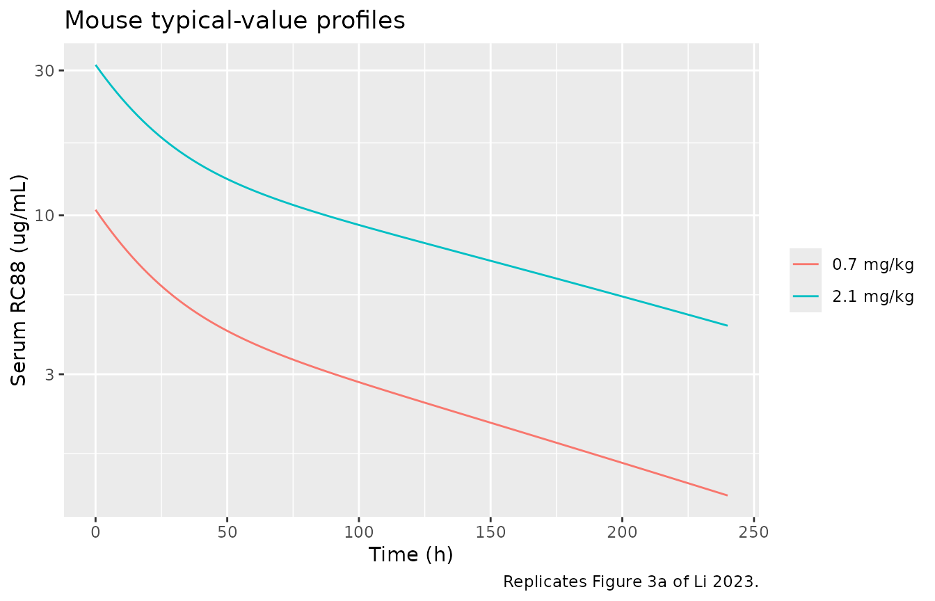
nca_input <- function(sim) {
  sim |>
    filter(!is.na(Cc)) |>
    select(id, time, Cc, treatment) |>
    distinct(id, time, .keep_all = TRUE)
}
dose_frame <- function(ev) {
  ev |> filter(evid == 1) |> select(id, time, amt, treatment)
}
run_nca <- function(sim, ev, end) {
  conc <- PKNCAconc(nca_input(sim), Cc ~ time | treatment + id)
  dose <- PKNCAdose(dose_frame(ev), amt ~ time | treatment + id, route = "intravascular")
  intervals <- data.frame(start = 0, end = end, cmax = TRUE, auclast = TRUE)
  as.data.frame(pk.nca(PKNCAdata(conc, dose, intervals = intervals)))
}
nca_mouse <- run_nca(sim_mouse, ev_mouse, 240)

ref_mouse <- data.frame(
  treatment = c("0.7 mg/kg", "2.1 mg/kg"),
  cmax = c(9.12, 36.5),
  auclast = c(418, 2118)
)
nlmixr2lib::ncaComparisonTable(
  nca_mouse, ref_mouse,
  by = "treatment", units = c(cmax = "ug/mL", auclast = "h*ug/mL"), tolerance_pct = 20
) |>
  dplyr::rename("Dose" = treatment) |>
knitr::kable(caption = "Mouse NCA (0-240 h) versus Li 2023 Table S1 (observed). * differs by more than 20%.", digits = 3)| NCA parameter | Dose | Reference | Simulated | % diff |
|---|---|---|---|---|
| Cmax (ug/mL) | 0.7 mg/kg | 9.12 | 10.4 | +14.4% |
| Cmax (ug/mL) | 2.1 mg/kg | 36.5 | 31.3 | -14.3% |
| AUClast (h*ug/mL) | 0.7 mg/kg | 418 | 751 | +79.7%* |
| AUClast (h*ug/mL) | 2.1 mg/kg | 2120 | 2430 | +14.6% |
Cmax is within 15% of Table S1. AUC at 0.7 mg/kg is about 1.8-fold above the observed value and AUC at 2.1 mg/kg about 15% above it: the printed typical values eliminate RC88 more slowly than the observed data, most visibly at the low dose where the Michaelis-Menten pathway matters most. The Michaelis-Menten units question behind this is discussed under Assumptions and deviations.
Monkey PK (Figure 3b, Table S1)
mod_monkey <- readModelDb("Li_2023_RC88_monkey")
doses_monkey <- c(0.5, 1.5, 5)
ev_monkey <- bind_rows(lapply(seq_along(doses_monkey), function(i) {
  bind_rows(
    data.frame(id = i, time = 0, amt = doses_monkey[i], evid = 1, cmt = "central"),
    data.frame(id = i, time = sort(unique(c(0, 0.083, 0.25, 2, 6, seq(0, 672, by = 4)))), amt = 0, evid = 0, cmt = "central")
  ) |>
    mutate(treatment = paste(doses_monkey[i], "mg/kg"))
}))
sim_monkey <- rxSolve(mod_monkey, ev_monkey, keep = "treatment") |> as.data.frame()
#> Warning: multi-subject simulation without without 'omega'

ggplot(sim_monkey, aes(time, Cc, colour = treatment)) +
  geom_line() +
  scale_y_log10() +
  labs(x = "Time (h)", y = "Serum RC88 (ug/mL)", colour = NULL,
       title = "Cynomolgus monkey typical-value profiles", caption = "Replicates Figure 3b of Li 2023.")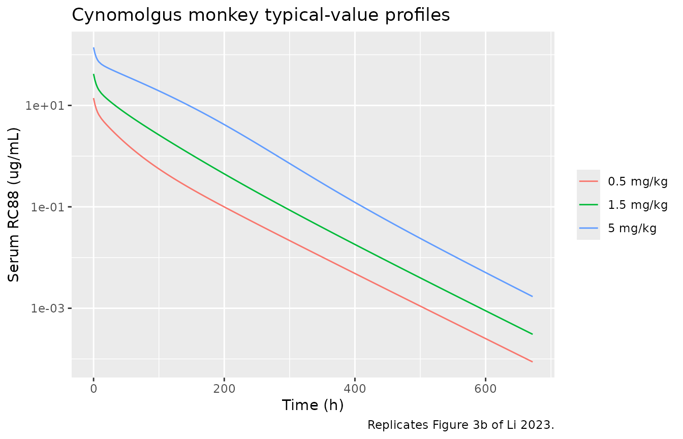
nca_monkey <- run_nca(sim_monkey, ev_monkey, 672)
ref_monkey <- data.frame(
  treatment = c("0.5 mg/kg", "1.5 mg/kg", "5 mg/kg"),
  cmax = c(14.7, 42.8, 132),
  auclast = c(332, 1097, 5777)
)
cmp_monkey <- nlmixr2lib::ncaComparisonTable(
  nca_monkey, ref_monkey,
  by = "treatment", units = c(cmax = "ug/mL", auclast = "h*ug/mL"), tolerance_pct = 20
)
cmp_monkey |>
  dplyr::rename("Dose" = treatment) |>
knitr::kable(caption = "Monkey NCA (0-672 h) versus Li 2023 Table S1 (observed means). * differs by more than 20%.", digits = 3)| NCA parameter | Dose | Reference | Simulated | % diff |
|---|---|---|---|---|
| Cmax (ug/mL) | 0.5 mg/kg | 14.7 | 14 | -5.0% |
| Cmax (ug/mL) | 1.5 mg/kg | 42.8 | 41.9 | -2.1% |
| Cmax (ug/mL) | 5 mg/kg | 132 | 140 | +5.8% |
| AUClast (h*ug/mL) | 0.5 mg/kg | 332 | 301 | -9.3% |
| AUClast (h*ug/mL) | 1.5 mg/kg | 1100 | 1080 | -1.4% |
| AUClast (h*ug/mL) | 5 mg/kg | 5780 | 5540 | -4.1% |
# The TMDD fit reproduces the observed exposure of all three dose groups:
# the target-mediated pathway saturates with dose, so AUC rises 17-fold for a
# 10-fold dose range in both the data and the model.
monkey_auc <- nca_monkey |> filter(PPTESTCD == "auclast") |> arrange(treatment)
stopifnot(
  nrow(monkey_auc) == 3,
  all(abs(monkey_auc$PPORRES / ref_monkey$auclast - 1) < 0.15)
)
The model also captures the dose non-proportionality: 0.5 to 5 mg/kg is a 10-fold dose step and a 17-fold AUC step, both observed and simulated.
Human projection and efficacious dose (Table 4)
Li 2023 replaced the mouse PK in the TGI models by the projected human PK and chose the q1w dose that holds the tumor static. With a linear (Simeoni) kill term, stasis over a dosing interval needs the average concentration over the interval to equal the TSC; the paper’s Table 4 doses correspond exactly to the average concentration over the first week after a single dose, AUC(0-168 h)/168, matching each TSC.
mod_human <- readModelDb("Li_2023_RC88_human")
cavg_week1 <- function(dose) {
  ev <- bind_rows(
    data.frame(id = 1, time = 0, amt = dose, evid = 1, cmt = "central"),
    data.frame(id = 1, time = seq(0, 168, by = 0.25), amt = 0, evid = 0, cmt = "central")
  )
  s <- rxSolve(mod_human, ev) |> as.data.frame() |> distinct(time, .keep_all = TRUE)
  sum(diff(s$time) * (head(s$Cc, -1) + tail(s$Cc, -1)) / 2) / 168
}
dose_for_tsc <- function(tsc) {
  uniroot(function(d) cavg_week1(d) - tsc, c(0.1, 10), tol = 1e-5)$root
}

table4 <- tibble::tribble(
  ~label,                        ~tsc, ~published_dose,
  "OVCAR3-MSLN-3# median",       1.84, 1.2,
  "OVCAR3-MSLN-3# lower",        1.22, 0.82,
  "OVCAR3-MSLN-3# upper",        2.32, 1.45,
  "H292-MSLN-9C8 median",        2.38, 1.5,
  "H292-MSLN-9C8 lower",         1.31, 0.88,
  "H292-MSLN-9C8 upper",         3.27, 1.96
) |>
  mutate(
    simulated_dose = vapply(tsc, dose_for_tsc, numeric(1)),
    pct_diff = 100 * (simulated_dose / published_dose - 1)
  )

table4 |>
  dplyr::rename(
    "Cell line / TSC" = label, "TSC (ug/mL)" = tsc,
    "Table 4 dose (mg/kg q1w)" = published_dose,
    "Simulated dose (mg/kg q1w)" = simulated_dose, "% diff" = pct_diff
  ) |>
knitr::kable(digits = 2, caption = "Weekly dose whose first-week average concentration equals the TSC, versus Li 2023 Table 4.")| Cell line / TSC | TSC (ug/mL) | Table 4 dose (mg/kg q1w) | Simulated dose (mg/kg q1w) | % diff |
|---|---|---|---|---|
| OVCAR3-MSLN-3# median | 1.84 | 1.20 | 1.21 | 0.42 |
| OVCAR3-MSLN-3# lower | 1.22 | 0.82 | 0.83 | 1.61 |
| OVCAR3-MSLN-3# upper | 2.32 | 1.45 | 1.47 | 1.57 |
| H292-MSLN-9C8 median | 2.38 | 1.50 | 1.51 | 0.34 |
| H292-MSLN-9C8 lower | 1.31 | 0.88 | 0.89 | 1.04 |
| H292-MSLN-9C8 upper | 3.27 | 1.96 | 1.96 | -0.15 |
# Deterministic solve against a printed table rounded to 2-3 digits.
stopifnot(all(abs(table4$pct_diff) < 5))
ev_h <- bind_rows(
  data.frame(id = 1, time = 168 * (0:3), amt = 1.2, evid = 1, cmt = "central"),
  data.frame(id = 1, time = seq(0, 672, by = 2), amt = 0, evid = 0, cmt = "central")
)
sim_h <- rxSolve(mod_human, ev_h) |> as.data.frame()
ggplot(sim_h, aes(time, Cc)) +
  geom_line() +
  geom_hline(yintercept = 1.84, linetype = 2) +
  scale_y_log10() +
  labs(x = "Time (h)", y = "Serum RC88 (ug/mL)",
       title = "Projected human profile, 1.2 mg/kg q1w x 4",
       caption = "Dashed line: OVCAR3-MSLN-3# median TSC (Table 4).")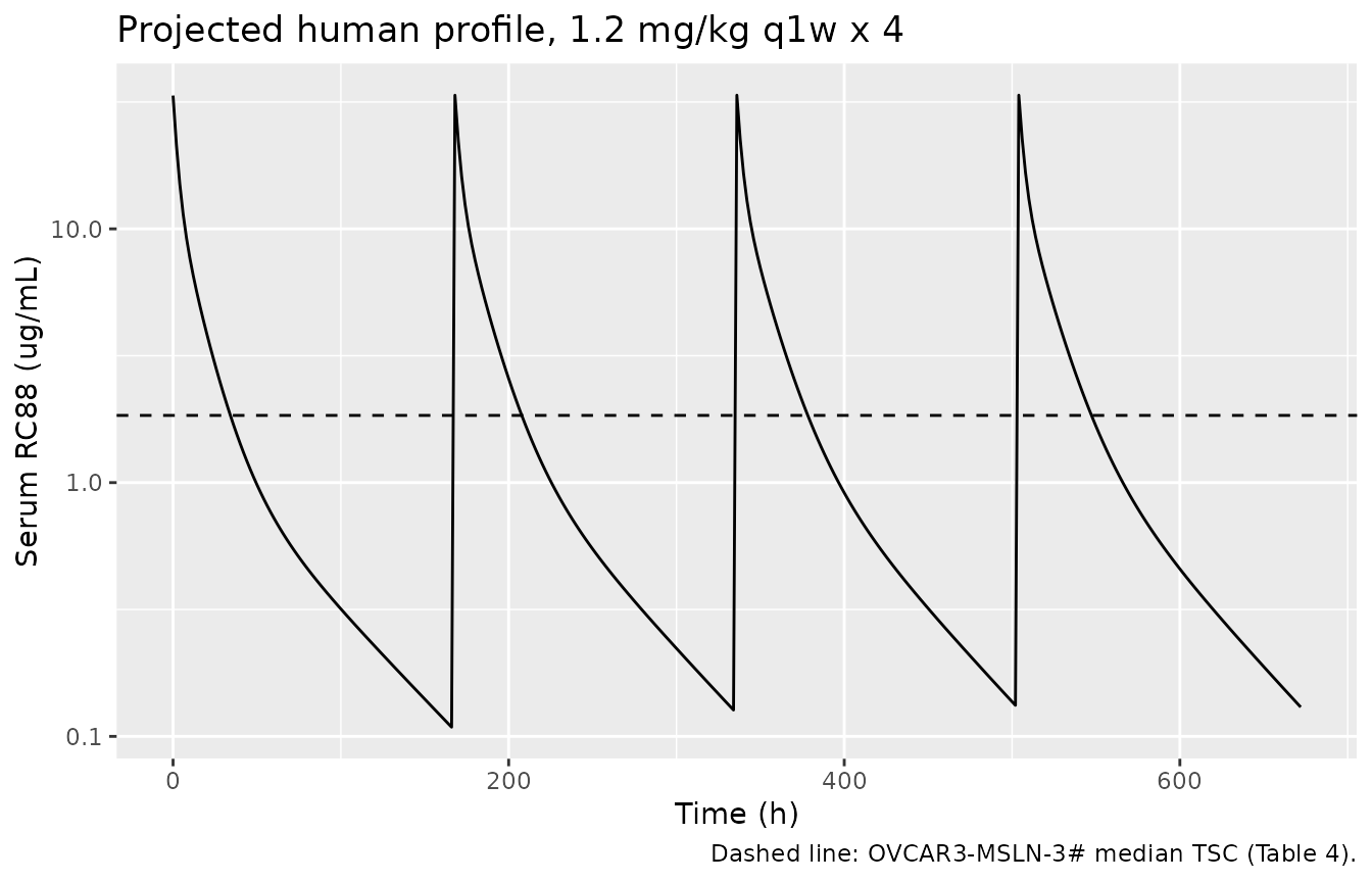
The projected human exposure is strongly target-mediated: baseline mesothelin (109.8 ug/mL drug-equivalent) far exceeds the concentration reached at these doses, so the trough at the end of each week is well below the TSC even though the weekly average matches it.
Tumor static concentration (Table 3)
Equation 4 gives the TSC for each TGI fit. The Simeoni and Jumbe values do not depend on tumor size; the Hybrid value does, and is evaluated here at the 250 mm^3 staging volume.
tsc_tab <- tibble::tribble(
  ~model,    ~study,           ~published,
  "simeoni", "ovcar3s",        1.84,
  "simeoni", "ovcar3m",        1.95,
  "simeoni", "h292",           3.27,
  "jumbe",   "ovcar3s",        1.22,
  "jumbe",   "h292",           2.38,
  "hybrid",  "ovcar3s",        2.32,
  "hybrid",  "ovcar3m",        1.37,
  "hybrid",  "h292",           1.31
)
tsc_from_model <- function(model, study) {
  ini_df <- rxode2::rxode(readModelDb(paste0("Li_2023_RC88_", model, "_", study, "_mouse_tgi")))$iniDf
  p <- function(nm) exp(ini_df$est[ini_df$name == nm])
  switch(model,
    simeoni = p("ltumorExpGrowth") / p("ldrugSlope"),
    jumbe = p("lkgrow") * p("lkc50") / (p("ldamageTransit") * p("lkmax") - p("lkgrow")),
    hybrid = {
      e <- 250
      g <- p("ltumorExpGrowth") * (1 - e / p("ltsmax"))
      sw <- (1 + (p("ltumorExpGrowth") / p("ltumorLinGrowth") * e)^20)^(1 / 20)
      g * p("lkc50") / (p("lkmax") * sw - g)
    }
  )
}
tsc_tab <- tsc_tab |>
  rowwise() |>
  mutate(computed = tsc_from_model(model, study)) |>
  ungroup() |>
  mutate(pct_diff = 100 * (computed / published - 1))

tsc_tab |>
  dplyr::rename("Model" = model, "Study" = study, "Table 3 TSC (ug/mL)" = published,
                "TSC from Tables S2-S4 (ug/mL)" = computed, "% diff" = pct_diff) |>
knitr::kable(digits = 2)| Model | Study | Table 3 TSC (ug/mL) | TSC from Tables S2-S4 (ug/mL) | % diff |
|---|---|---|---|---|
| simeoni | ovcar3s | 1.84 | 1.87 | 1.83 |
| simeoni | ovcar3m | 1.95 | 2.03 | 3.97 |
| simeoni | h292 | 3.27 | 4.02 | 23.03 |
| jumbe | ovcar3s | 1.22 | 1.22 | 0.20 |
| jumbe | h292 | 2.38 | 2.40 | 0.76 |
| hybrid | ovcar3s | 2.32 | 2.42 | 4.30 |
| hybrid | ovcar3m | 1.37 | 1.15 | -15.94 |
| hybrid | h292 | 1.31 | 2.27 | 73.18 |
# The Jumbe TSC formula pins the reading of the Table S2 transit constant:
# multiplying Kkill by 0.107 returns the published 1.22 ug/mL, dividing by it
# would give 0.013 ug/mL.
jumbe_rows <- tsc_tab |> filter(model == "jumbe")
stopifnot(nrow(jumbe_rows) == 2, all(abs(jumbe_rows$pct_diff) < 2))
The Jumbe values reproduce Table 3. The Simeoni OVCAR3 values agree within 4%. The others are limited by how the tables are rounded. Table S3 prints lambda0 for H292 to one significant figure (0.007), and the Hybrid TSC denominator, Kmax - KgEx(1 - E/Emax), is a small difference of two rounded numbers (KgEx is printed to one significant figure). Neither can be closer than these roundings allow. Table 3 also reports the TSCs from the fitting software’s secondary-parameter output rather than from the rounded tables.
Tumor growth inhibition (Figure 2)
Each TGI model is solved at the doses of its study, starting from the mean initial tumor volume read from Figure 2 by the maintainers (about 340, 270 and 290 mm^3 for panels a, b and c). The points are the group means read from Figure 2.
solve_tgi <- function(stem, doses, n_doses, v0, tmax) {
  mod <- rxode2::rxode2(readModelDb(paste0("Li_2023_RC88_", stem, "_mouse_tgi"))) |>
    ini(lrbase_tumor = log(v0))
  bind_rows(lapply(seq_along(doses), function(i) {
    dose <- doses[i]
    obs <- data.frame(id = i, time = seq(0, tmax, by = 4), amt = 0, evid = 0, cmt = "central")
    ev <- if (dose > 0) {
      bind_rows(data.frame(id = i, time = 168 * (seq_len(n_doses) - 1), amt = dose, evid = 1, cmt = "central"), obs)
    } else {
      obs
    }
    rxSolve(mod, ev) |>
      as.data.frame() |>
      mutate(dose = if (dose > 0) paste(dose, "mg/kg") else "Control")
  })) |>
    mutate(model = sub("_.*", "", stem), study = sub(".*_", "", stem))
}

sim_a <- bind_rows(lapply(c("simeoni_ovcar3s", "jumbe_ovcar3s", "hybrid_ovcar3s"),
                          solve_tgi, doses = c(0, 0.7, 2.1), n_doses = 1, v0 = 340, tmax = 264))
#> ℹ change initial estimate of `lrbase_tumor` to `5.82894561761021`
#> ℹ change initial estimate of `lrbase_tumor` to `5.82894561761021`
#> ℹ change initial estimate of `lrbase_tumor` to `5.82894561761021`
sim_b <- bind_rows(lapply(c("simeoni_ovcar3m", "hybrid_ovcar3m"),
                          solve_tgi, doses = c(0, 0.75, 1.5, 3), n_doses = 3, v0 = 270, tmax = 504))
#> ℹ change initial estimate of `lrbase_tumor` to `5.59842195899838`
#> ℹ change initial estimate of `lrbase_tumor` to `5.59842195899838`
sim_c <- bind_rows(lapply(c("simeoni_h292", "jumbe_h292", "hybrid_h292"),
                          solve_tgi, doses = c(0, 0.75, 1.5, 3), n_doses = 3, v0 = 290, tmax = 504))
#> ℹ change initial estimate of `lrbase_tumor` to `5.66988092298052`
#> ℹ change initial estimate of `lrbase_tumor` to `5.66988092298052`
#> ℹ change initial estimate of `lrbase_tumor` to `5.66988092298052`

# Group means read from Li 2023 Figure 2 by the maintainers.
fig2 <- bind_rows(
  tibble::tribble(
    ~dose,       ~time, ~tumor_vol,
    "Control",   48,  470, "Control",  96,  580, "Control",  168, 715, "Control",  264, 880,
    "0.7 mg/kg", 48,  470, "0.7 mg/kg", 96, 450, "0.7 mg/kg", 168, 390, "0.7 mg/kg", 264, 405,
    "2.1 mg/kg", 48,  405, "2.1 mg/kg", 96, 300, "2.1 mg/kg", 168, 110, "2.1 mg/kg", 264, 60
  ) |> mutate(panel = "a"),
  tibble::tribble(
    ~dose,        ~time, ~tumor_vol,
    "Control",    72, 440, "Control",    168, 760, "Control",    240, 920,
    "Control",    336, 1020, "Control",  408, 1270, "Control",   504, 1660,
    "0.75 mg/kg", 72, 390, "0.75 mg/kg", 168, 340, "0.75 mg/kg", 240, 410,
    "0.75 mg/kg", 336, 560, "0.75 mg/kg", 408, 850, "0.75 mg/kg", 504, 1170,
    "1.5 mg/kg",  72, 300, "1.5 mg/kg",  168, 120, "1.5 mg/kg",  240, 80,
    "1.5 mg/kg",  336, 20, "1.5 mg/kg",  408, 5, "1.5 mg/kg",    504, 5,
    "3 mg/kg",    72, 240, "3 mg/kg",    168, 30, "3 mg/kg",     240, 5,
    "3 mg/kg",    336, 0, "3 mg/kg",     408, 0, "3 mg/kg",      504, 0
  ) |> mutate(panel = "b"),
  tibble::tribble(
    ~dose,        ~time, ~tumor_vol,
    "Control",    72, 530, "Control",    168, 840, "Control",    240, 1130,
    "Control",    336, 1500, "Control",  408, 2100, "Control",   504, 2650,
    "0.75 mg/kg", 72, 420, "0.75 mg/kg", 168, 700, "0.75 mg/kg", 240, 900,
    "0.75 mg/kg", 336, 1100, "0.75 mg/kg", 408, 1080, "0.75 mg/kg", 504, 1300,
    "1.5 mg/kg",  72, 380, "1.5 mg/kg",  168, 400, "1.5 mg/kg",  240, 480,
    "1.5 mg/kg",  336, 530, "1.5 mg/kg", 408, 660, "1.5 mg/kg",  504, 740,
    "3 mg/kg",    72, 340, "3 mg/kg",    168, 290, "3 mg/kg",    240, 250,
    "3 mg/kg",    336, 230, "3 mg/kg",   408, 240, "3 mg/kg",    504, 200
  ) |> mutate(panel = "c")
)

plot_panel <- function(sim, p, title) {
  ggplot(sim, aes(time, tumor_vol, colour = dose)) +
    geom_line(aes(linetype = model)) +
    geom_point(data = filter(fig2, panel == p), aes(time, tumor_vol, colour = dose), inherit.aes = FALSE) +
    labs(x = "Time (h)", y = "Tumor volume (mm^3)", colour = NULL, linetype = NULL, title = title)
}
plot_panel(sim_a, "a", "OVCAR3-MSLN-3#, single dose") +
  labs(caption = "Replicates Figure 2a of Li 2023 (lines: models; points: Figure 2 means).")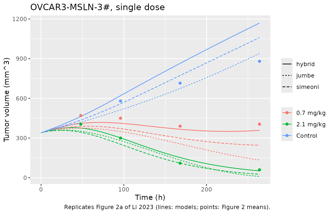
plot_panel(sim_b, "b", "OVCAR3-MSLN-3#, q1w x 3") +
  labs(caption = "Replicates Figure 2b of Li 2023 (lines: models; points: Figure 2 means).")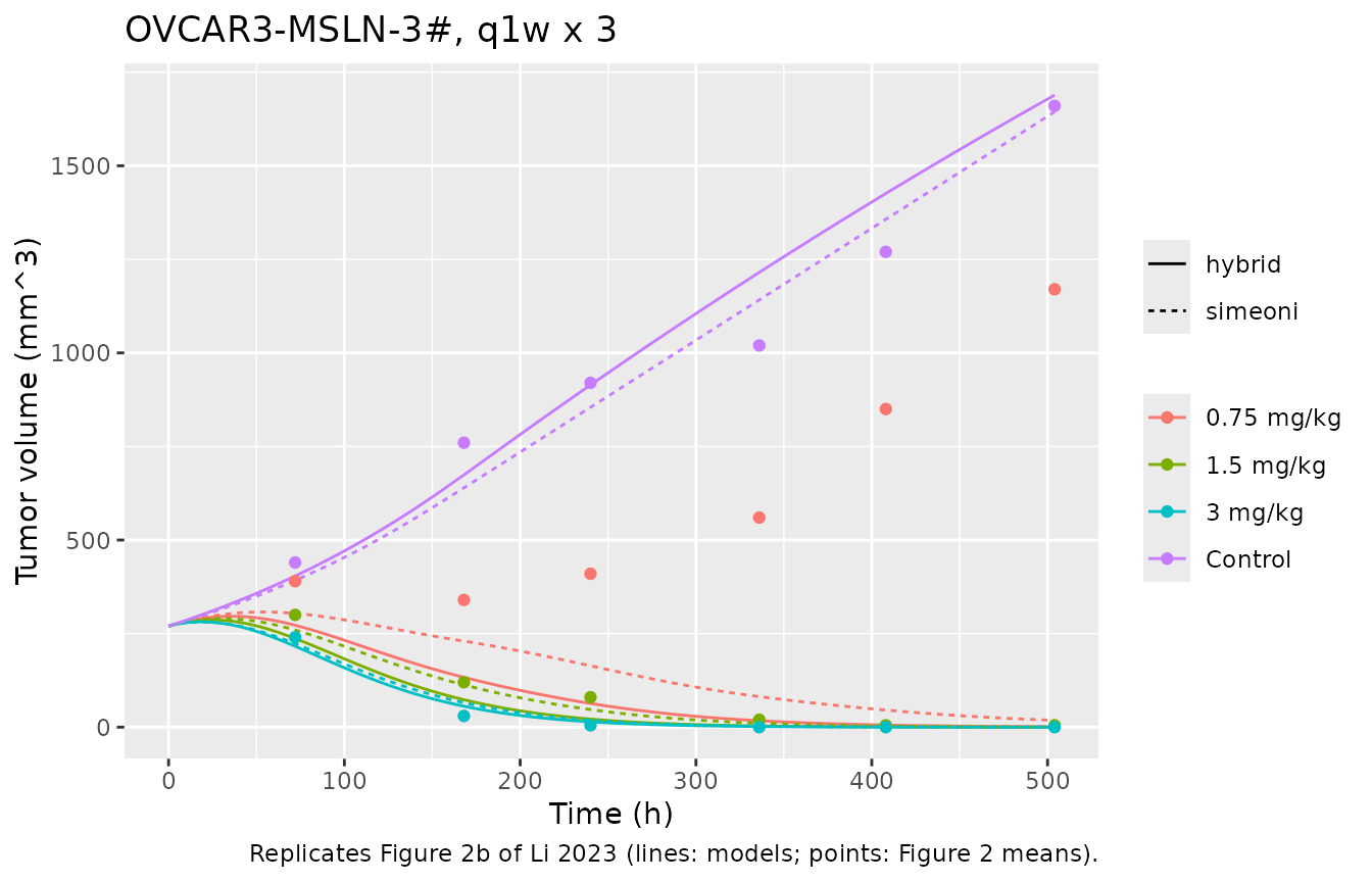
plot_panel(sim_c, "c", "H292-MSLN-9C8, q1w x 3") +
  labs(caption = "Replicates Figure 2c of Li 2023 (lines: models; points: Figure 2 means).")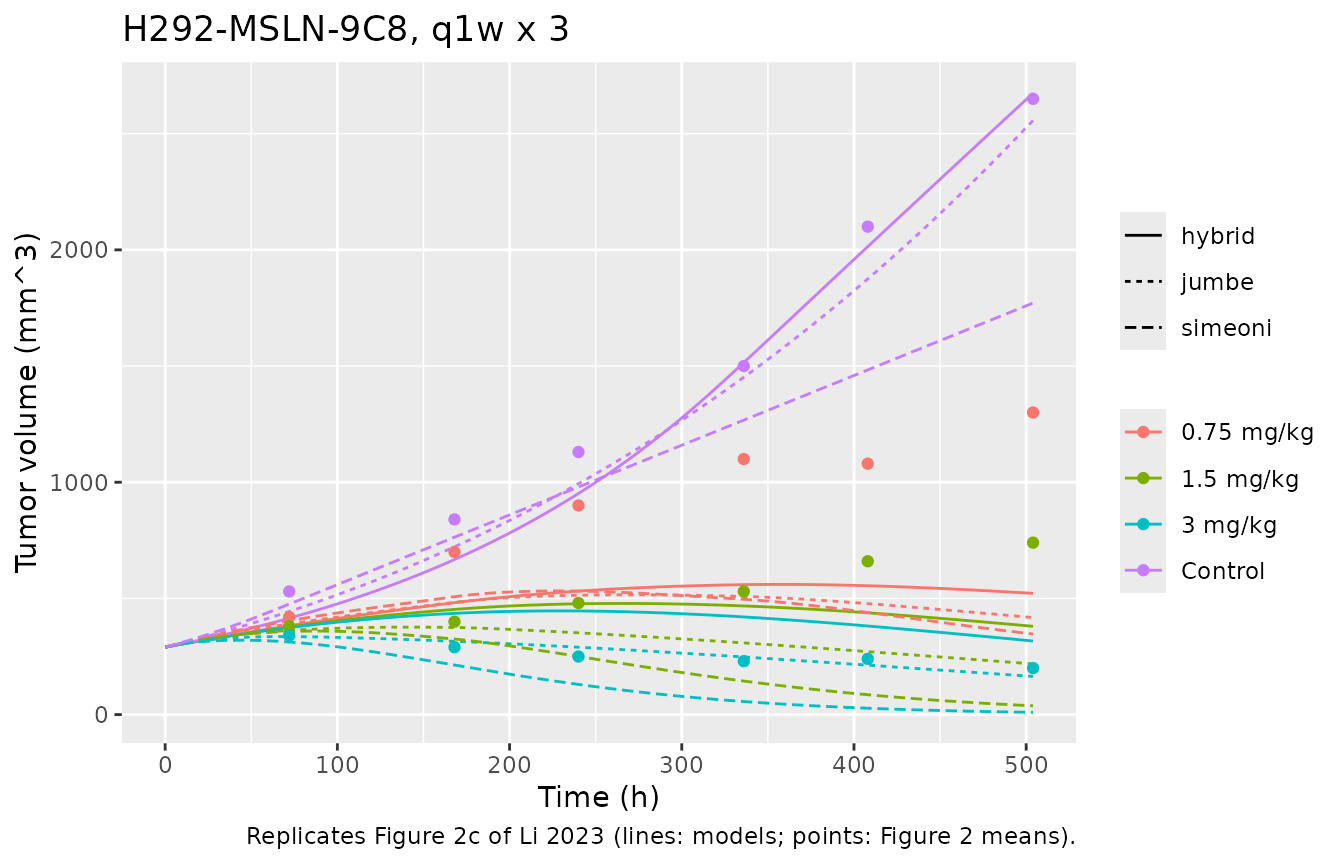
# Structural checks that hold whatever the PK reading: every control arm
# grows, and every model ranks its dose arms in order at the end of the study.
end_vol <- bind_rows(sim_a, sim_b, sim_c) |>
  group_by(model, study, dose) |>
  filter(time == max(time)) |>
  ungroup() |>
  mutate(dose_num = ifelse(dose == "Control", 0, as.numeric(sub(" mg/kg", "", dose))))
#> Warning: There was 1 warning in `mutate()`.
#> ℹ In argument: `dose_num = ifelse(dose == "Control", 0, as.numeric(sub("
#>   mg/kg", "", dose)))`.
#> Caused by warning in `ifelse()`:
#> ! NAs introduced by coercion
# 3 models x 3 arms (panel a) + 2 models x 4 arms (b) + 3 models x 4 arms (c)
stopifnot(nrow(end_vol) == 29)
v0_by_study <- c(ovcar3s = 340, ovcar3m = 270, h292 = 290)
ranked <- end_vol |>
  group_by(model, study) |>
  arrange(dose_num, .by_group = TRUE) |>
  summarise(
    control_grows = tumor_vol[dose_num == 0] > 2 * v0_by_study[[study[1]]],
    monotone = all(diff(tumor_vol) <= 1e-6 * max(tumor_vol)),
    .groups = "drop"
  )
stopifnot(nrow(ranked) == 8, all(ranked$control_grows), all(ranked$monotone))
Every model reproduces the single-dose OVCAR3-MSLN-3# study (panel a), the regressions at 1.5 and 3 mg/kg in the multiple-dose OVCAR3-MSLN-3# study (panel b), and the 3 mg/kg H292-MSLN-9C8 arm (panel c). The control arms are reproduced except the Simeoni H292-MSLN-9C8 fit, which reaches about 1800 mm^3 at 504 h against an observed 2650 mm^3. The fits differ from Figure 2 at the partially effective doses: 0.75 mg/kg in panel b, and 0.75 and 1.5 mg/kg in panel c. There the models predict more tumor shrinkage than was observed. Two things limit agreement at those doses. These are typical-value models with no interindividual variability (Figure 2 shows group means). The low-dose mouse exposure also depends on the Michaelis-Menten units question described below.
Assumptions and deviations
- Mouse Vmax units. Table 2 labels the mouse Vmax “ug/mL/h”. Read as a concentration rate (amount rate Vmax x V1), the Michaelis-Menten pathway alone removes RC88 with a 2-h half-life at low concentrations. Serum RC88 after 0.7 mg/kg then falls to about 0.06 ug/mL at 24 h. Figure 3a shows about 5 ug/mL at 24 h, with RC88 still measurable at 240 h. That reading also gives AUCs about 7-fold below Table S1, and loses the 2.1 mg/kg regression in Figure 2a. Vmax is therefore encoded as an amount rate per kg body weight (ug/h/kg), dimensionally consistent with the per-kg doses and volumes. Under this reading Cmax matches Table S1 and AUC is 15% (2.1 mg/kg) to 80% (0.7 mg/kg) above it, so the true low-concentration elimination lies between the two readings. No scale factor was fitted.
-
Variability. The paper reports no interindividual
or residual variability for any fit (Phoenix NLME, FOCE-ELS). Every
model therefore carries a single
fixed(0)proportional residual error and no etas; it simulates the typical value only. - Simeoni growth term. Equation 1 uses E1 (cycling cells) in both the numerator and the exponential-to-linear switch. The original Simeoni 2004 model uses total tumor weight in the switch. The printed equation is encoded.
-
Jumbe transit constant. Table S2 calls
ta “transit rate constant” with unit “(h)”, and Equation 3 prints 1/t. The tabulated value is used wherever Equation 3 prints 1/t, because only this reading makes the paper’s TSC formula return its Table 3 TSCs (1.22 and 2.38 ug/mL). The Jumbe growth constant Kgrow is labelled 1/h but multiplies volume^(2/3), as printed. -
Jumbe non-negativity. A rate proportional to
volume^(2/3) can empty a compartment in finite time. Each volume^(2/3)
term is evaluated on
max(state, 0)so an emptied compartment stays at zero, where the equations are undefined below zero. - Initial tumor volume. The paper used each animal’s measured volume as the E1 initial condition. The models default to the 250 mm^3 staging volume; this article overrides it with the Figure 2 group means.
- H292 PK. The mouse PK was measured in OVCAR3-MSLN-3# tumor-bearing mice. The paper fixed the same PK for the H292-MSLN-9C8 fits, and the models do the same.
- Text discrepancies. The Results text gives the top monkey dose as 3 mg/kg; Methods, Figure 3b and Table S1 all give 5 mg/kg, which is used here. Table 1 lists 3 animals per group for the single-dose OVCAR3 study; the Methods text says 6. Table S3 prints identical lambda0 and RSE for the OVCAR3 (S) and (M) Simeoni fits.
- Human projection. All human parameters are fixed scaled values (allometric exponent 1 on the per-kg clearances and volumes, rate constants 1:1, baseline mesothelin x3 for disease). They are not estimates from human data.