Epinephrine (Abboud 2009)
Source:vignettes/articles/Abboud_2009_epinephrine.Rmd
Abboud_2009_epinephrine.RmdModel and source
- Citation: Abboud I, Lerolle N, Urien S, Tadie JM, Leviel F, Fagon JY, Faisy C. Pharmacokinetics of epinephrine in patients with septic shock: modelization and interaction with endogenous neurohormonal status. Crit Care 2009;13(4):R120. doi:10.1186/cc7972.
- Description: One-compartment population PK model for intravenous epinephrine (adrenaline) infusion in adults with septic shock, with a constant endogenous epinephrine production rate (R0) feeding the central compartment and body weight and SAPS II severity score as power covariates on clearance (Abboud 2009).
- Article: https://doi.org/10.1186/cc7972 (open access in Critical Care 2009;13:R120)
Population
Thirty-eight consecutive adult patients with septic shock were enrolled prospectively at the medical ICU of Hopital Europeen Georges Pompidou (Paris, France) between January and June 2006 and provided 73 plasma epinephrine concentrations for the population PK analysis. Baseline demographics are reproduced from Table 1 of the source: mean age 64 +/- 15 years, mean body weight 68 +/- 19 kg, 65.7 percent male, mean SAPS II score at ICU admission 64 +/- 23, median 1 day in the ICU before inclusion (range 1-22), 65.7 percent ICU mortality. The leading causes of septic shock were pneumonia (community-acquired 10, nosocomial 12), intra-abdominal infection (6), mediastinitis (4), other (4), and undocumented (2).
The same information is available programmatically via the model’s
population metadata
(readModelDb("Abboud_2009_epinephrine")$population).
Source trace
The per-parameter origin is recorded as an in-file comment next to
each ini() entry in
inst/modeldb/specificDrugs/Abboud_2009_epinephrine.R. The
table below collects them in one place for review.
| Equation / parameter | Value | Source location |
|---|---|---|
lcl (CL at reference) |
127 L/h | Table 3 row “CL (L/hr/70 kg BW/50 SAPS II units)” |
lvc (V) |
7.9 L | Table 3 row “V (L)” |
lr0 (R0) |
43.5 nmol/h | Table 3 row “R0 (nmol/h)” |
e_wt_cl (WT exponent on CL) |
0.60 | Table 3 row “theta_BW effect on CL” |
e_saps_ii_cl (SAPS II exponent on CL) |
-0.67 | Table 3 row “theta_SAPS II effect on CL” |
etalcl variance |
0.33^2 = 0.1089 | Table 3 row “BSV(CL)” (reports SD = sqrt(omega^2)) |
etalr0 variance |
1.23^2 = 1.5129 | Table 3 row “BSV(R0)” (reports SD = sqrt(omega^2)) |
propSd (FIXED) |
0.10 | Table 3 row “Residual variability, proportional component” with footnote “b Fixed values”; Methods “the residual variability parameters were fixed as follows: 10% and 0.1 nmol/L” |
addSd (FIXED) |
0.10 nmol/L | Table 3 row “Residual variability, additive component”; same Methods quotation |
d/dt(central) |
r0 - kel * central |
Results: one-compartment open model with first-order elimination; Methods statement that R0 “allowed us to take into account the baseline epinephrine concentration at C0” |
central(0) |
r0 / kel |
Pre-infusion steady-state under endogenous production alone (Methods); reproduces the C0 measurement |
Cc_plateau |
(rate + R0) / CL |
Results explicit formula:
C_plateau (nmol/L) = (rate of infusion + R0) / (127 * (BW/70)^0.60 * (SAPS II/50)^-0.67)
|
Virtual cohort
Original individual data are not publicly available. The cohort below uses covariate distributions matching the published Table 1 / Table 2 summaries: 38 subjects with body weight ~ Normal(68, 19) kg (truncated to physiological range), SAPS II ~ Normal(64, 23) (truncated to 0-120), and per-subject steady- state infusion rates drawn to span the observed 100-fold range at the C1 sampling point (0.026 to 1.7 ug/kg/min).
set.seed(20090720)  # paper publication date

n_subj <- 38L

# Per-subject covariates and infusion rates drawn to approximate the reported
# distributions. Truncate body weight and SAPS II to a defensible range.
cohort <- tibble(
  id      = seq_len(n_subj),
  WT      = pmax(40, pmin(120, round(rnorm(n_subj, mean = 68, sd = 19)))),
  SAPS_II = pmax(20, pmin(110, round(rnorm(n_subj, mean = 64, sd = 23)))),
  # Steady-state IV infusion rate at C1 sampling, ug/kg/min on a log-uniform
  # grid spanning the observed 100-fold range (Table 2).
  rate_ug_per_kg_per_min = exp(seq(log(0.026), log(1.7), length.out = n_subj))
) |>
  mutate(
    # Convert rate to nmol/h for the model:
    #   ug/kg/min * WT (kg) * 60 min/h / 0.1832 (ug/nmol) = nmol/h
    # because 1 nmol epinephrine = 0.1832 ug (MW 183.2 g/mol).
    rate_nmol_per_h = rate_ug_per_kg_per_min * WT * 60 / 0.1832,
    rate_mg_per_h   = rate_ug_per_kg_per_min * WT * 60 / 1000
  )

knitr::kable(
  head(cohort, 6) |> mutate(across(where(is.numeric), ~ signif(.x, 3))),
  caption = "First six simulated subjects (body weight, SAPS II, infusion rate)."
)| id | WT | SAPS_II | rate_ug_per_kg_per_min | rate_nmol_per_h | rate_mg_per_h |
|---|---|---|---|---|---|
| 1 | 77 | 110 | 0.0260 | 656 | 0.1200 |
| 2 | 80 | 75 | 0.0291 | 763 | 0.1400 |
| 3 | 93 | 93 | 0.0326 | 993 | 0.1820 |
| 4 | 70 | 34 | 0.0365 | 837 | 0.1530 |
| 5 | 40 | 38 | 0.0409 | 535 | 0.0981 |
| 6 | 41 | 57 | 0.0457 | 614 | 0.1130 |
Simulation
A 12-hour continuous IV infusion is more than long enough to reach steady state for a drug with a plasma half-life of about 3.5 minutes. The simulation samples the plateau concentration at 6 hours.
mod <- readModelDb("Abboud_2009_epinephrine")

# Build one-row-per-subject dose + observation events.
# Dose: rate column carries the infusion rate (nmol/h); duration is set long
# enough that the plateau is reached well before the observation time.
# Observation: a single Cc reading at t = 6 hours.
dose_rows <- cohort |>
  transmute(
    id   = id,
    time = 0,
    amt  = rate_nmol_per_h * 12,   # total nmol over 12-hour infusion
    rate = rate_nmol_per_h,
    evid = 1L,
    cmt  = "central",
    WT, SAPS_II
  )

obs_rows <- cohort |>
  transmute(
    id   = id,
    time = 6,
    amt  = 0,
    rate = 0,
    evid = 0L,
    cmt  = "central",
    WT, SAPS_II
  )

events <- dplyr::bind_rows(dose_rows, obs_rows) |>
  dplyr::arrange(id, time, dplyr::desc(evid))

# Typical-value simulation (no between-subject variability) to recover the
# Results formula exactly.
mod_typical <- mod |> rxode2::zeroRe()
#> ℹ parameter labels from comments will be replaced by 'label()'
sim_typical <- rxode2::rxSolve(
  mod_typical, events = events, keep = c("WT", "SAPS_II"),
  addDosing = FALSE
) |>
  as.data.frame()
#> ℹ omega/sigma items treated as zero: 'etalcl', 'etalrbase'
#> Warning: multi-subject simulation without without 'omega'
Replicate published Table 3 / Figure 1 (steady-state plateau)
The paper’s explicit prediction formula is
C_plateau (nmol/L) = (rate + R0) / [127 * (BW/70)^0.60 * (SAPS_II/50)^-0.67]For the typical-value simulation (no eta), the model’s
Cc at the plateau time should match this formula
exactly.
plateau <- sim_typical |>
  dplyr::filter(time == 6) |>
  dplyr::select(id, WT, SAPS_II, Cc_model = Cc) |>
  dplyr::left_join(
    cohort |> dplyr::select(id, rate_nmol_per_h, rate_ug_per_kg_per_min),
    by = "id"
  ) |>
  dplyr::mutate(
    cl_typical    = 127 * (WT / 70)^0.60 * (SAPS_II / 50)^-0.67,
    Cc_formula    = (rate_nmol_per_h + 43.5) / cl_typical,
    abs_rel_error = abs(Cc_model - Cc_formula) / Cc_formula
  )

knitr::kable(
  head(plateau, 6) |> dplyr::mutate(dplyr::across(where(is.numeric), ~ signif(.x, 4))),
  caption = "Per-subject simulated plateau Cc compared with the paper's explicit prediction formula."
)| id | WT | SAPS_II | Cc_model | rate_nmol_per_h | rate_ug_per_kg_per_min | cl_typical | Cc_formula | abs_rel_error |
|---|---|---|---|---|---|---|---|---|
| 1 | 77 | 110 | 8.818 | 655.7 | 0.02600 | 79.29 | 8.818 | 0 |
| 2 | 80 | 75 | 7.688 | 762.7 | 0.02911 | 104.90 | 7.688 | 0 |
| 3 | 93 | 93 | 10.430 | 992.7 | 0.03259 | 99.37 | 10.430 | 0 |
| 4 | 70 | 34 | 5.352 | 836.6 | 0.03649 | 164.40 | 5.352 | 0 |
| 5 | 40 | 38 | 5.304 | 535.2 | 0.04085 | 109.10 | 5.304 | 0 |
| 6 | 41 | 57 | 7.794 | 614.2 | 0.04574 | 84.39 | 7.794 | 0 |
cat(sprintf(
  "Maximum absolute relative error between simulated plateau and formula: %g\n",
  max(plateau$abs_rel_error)
))
#> Maximum absolute relative error between simulated plateau and formula: 1.34644e-09

stopifnot(max(plateau$abs_rel_error) < 1e-3)
# Build a dense grid of (rate, WT, SAPS_II) and overlay model predictions with
# the closed-form formula to show the model behaviour Abboud 2009 Figure 1
# illustrates (observed vs predicted plateau concentrations).
grid <- tidyr::expand_grid(
  rate_ug_per_kg_per_min = exp(seq(log(0.026), log(1.7), length.out = 60)),
  WT                     = c(50, 70, 90),
  SAPS_II                = c(40, 60, 80)
) |>
  dplyr::mutate(
    rate_nmol_per_h = rate_ug_per_kg_per_min * WT * 60 / 0.1832,
    cl_typical     = 127 * (WT / 70)^0.60 * (SAPS_II / 50)^-0.67,
    Cc_plateau     = (rate_nmol_per_h + 43.5) / cl_typical,
    saps_label     = paste0("SAPS II = ", SAPS_II)
  )

ggplot(grid, aes(rate_ug_per_kg_per_min, Cc_plateau, colour = factor(WT))) +
  geom_line() +
  facet_wrap(~ saps_label) +
  scale_x_log10() +
  scale_y_log10() +
  labs(
    x      = "Epinephrine infusion rate (ug/kg/min)",
    y      = "Plateau plasma epinephrine (nmol/L)",
    colour = "Body weight (kg)",
    title  = "Predicted epinephrine plateau vs. infusion rate",
    caption = "Reproduces the typical-value relationship behind Figure 1 of Abboud 2009."
  ) +
  theme_minimal()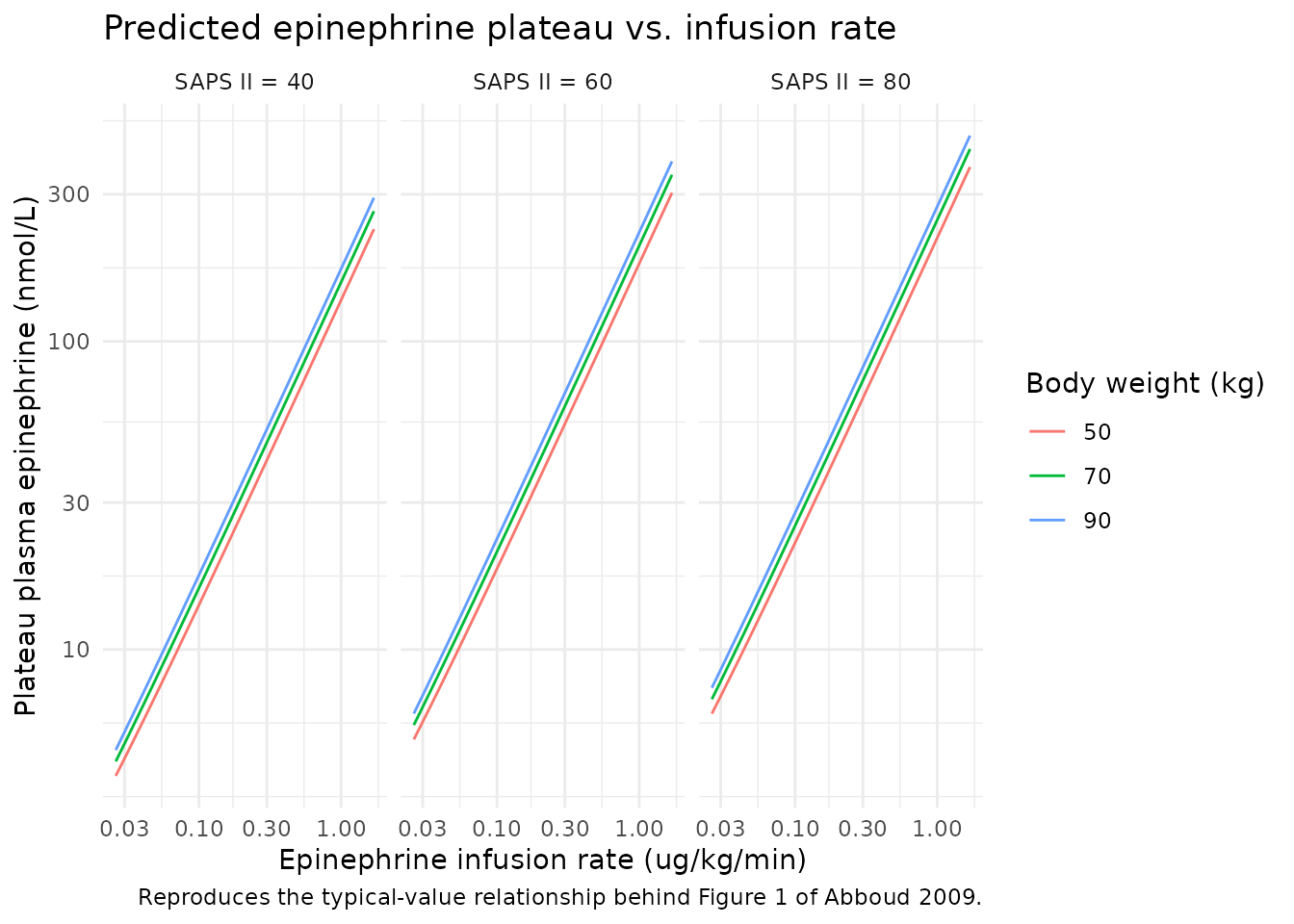
Replicates Figure 1 of Abboud 2009: typical-value epinephrine plateau concentration vs. infusion rate, faceted by representative SAPS II strata.
Steady-state and baseline checks (endogenous-model validation)
For this hybrid exogenous-infusion + endogenous-production model, the right validations are (i) the pre-infusion baseline (C0) reproduces the typical endogenous epinephrine concentration in Table 2, and (ii) the steady-state plateau under continuous infusion reproduces the explicit formula in the Results.
1. Pre-infusion baseline check
With no exogenous infusion, the initial condition
central(0) = r0 / kel means the model starts at the
endogenous steady state. The typical-subject baseline concentration
Cc(0) should equal R0 / CL_typical = 43.5 / 127 = 0.343 nmol/L, matching
the median baseline epinephrine of 0.34 nmol/L reported in Table 2.
ev_noinf <- rxode2::et(amt = 0, time = 0) |>
  rxode2::et(seq(0, 1, by = 0.05)) |>
  dplyr::as_tibble() |>
  dplyr::mutate(id = 1, WT = 70, SAPS_II = 50)

baseline_sim <- rxode2::rxSolve(
  mod_typical, events = ev_noinf
) |>
  as.data.frame()
#> ℹ omega/sigma items treated as zero: 'etalcl', 'etalrbase'

baseline_typical <- 43.5 / 127
cat(sprintf(
  "Typical-subject baseline Cc(0) = %.4f nmol/L (formula R0/CL = %.4f); Table 2 reports median 0.34 nmol/L.\n",
  baseline_sim$Cc[1], baseline_typical
))
#> Typical-subject baseline Cc(0) = 0.3425 nmol/L (formula R0/CL = 0.3425); Table 2 reports median 0.34 nmol/L.

stopifnot(abs(baseline_sim$Cc[1] - baseline_typical) < 1e-6)
2. Steady-state mass-balance check
At steady state under a constant exogenous infusion R_in
(nmol/h) and the constant endogenous production R0, the
central-compartment mass balance is
0 = R_in + R0 - kel * central_ssso central_ss = (R_in + R0) / kel and
Cc_ss = (R_in + R0) / CL. Verified numerically by the
plateau-check chunk above (max relative error <
1e-3).
3. Dimensional check
| Term | Unit |
|---|---|
r0 |
nmol/h |
kel * central |
(1/h) * nmol = nmol/h |
central / vc |
nmol / L = nmol/L (= Cc) |
exogenous rate (event column) |
nmol/h |
(rate + r0) / cl |
(nmol/h) / (L/h) = nmol/L |
Right-hand side of d/dt(central) and the closed-form
plateau are both nmol-per-hour and nmol-per-litre respectively,
consistent with the declared units list.
Assumptions and deviations
- Original individual-level data are not publicly available; the
virtual cohort approximates Table 1 / Table 2 summary statistics. Race /
ethnicity was not reported in the source and is omitted from
populationand from the simulated data. - The endogenous production rate
R0is modelled as time-invariant per the source paper. The paper notes that exogenous epinephrine altered norepinephrine metabolism (Table 2) but did not retain any time-varying R0 mechanism in the final PK model, so this file keeps R0 constant. - IIVs are assumed independent. Methods state that covariances “were also estimated” but the final-model Table 3 reports only the diagonal SDs and Methods explicitly says “if the correlation between terms was low, it was fixed at 0”, so no off-diagonal terms are introduced here.
- Residual error components are encoded with
fixed()because Methods and Table 3 footnote “b” explicitly mark them as fixed (proportional = 10 percent, additive = 0.1 nmol/L, both set to the HPLC assay quantification). - Comparison against published NCA is not applicable: the source paper did not report any NCA-style summary (Cmax / AUC / half-life apart from a derived typical half-life of 3.5 minutes), and the C1 sample is a single steady-state observation per patient. The validation here therefore uses steady-state algebraic equivalence to the published prediction formula, matching the endogenous-model validation pattern.