Rivaroxaban (Ren 2026) • nlmixr2lib

Model and source

#> ℹ parameter labels from comments will be replaced by 'label()'

Citation: Ren J, Li Y, Zheng X, Wu Z, Shi J, Han X. Population pharmacokinetic and pharmacodynamic analysis of rivaroxaban in real-world patients with pulmonary embolism in China. Res Pract Thromb Haemost. 2026;10:106618. doi:10.1016/j.rpth.2026.106618.
Description: Joint population pharmacokinetic-pharmacodynamic model for rivaroxaban in real-world Chinese adults treated for pulmonary embolism (Ren 2026). The PK layer is a one-compartment oral model with first-order absorption and elimination; creatinine clearance enters CL/F and age enters V/F, both as median-normalized power terms. The PD layer is a direct linear concentration-prothrombin time relationship, PT = baseline + slope * Cc, with alanine aminotransferase entering the slope as a median-normalized power term. The two endpoints (plasma rivaroxaban concentration and prothrombin time) are declared jointly; the authors fitted the PD layer sequentially on the PK posterior and then re-estimated the combined PK/PD model. Interindividual variability was not supported on ka (99.8% shrinkage) and was dropped by the authors.
Article: https://doi.org/10.1016/j.rpth.2026.106618

No supplementary material accompanies this article; every parameter below comes from the main text, Table 2 (PK) or Table 3 (PD).

Population

Ren 2026 is a single-centre prospective cohort of 187 Chinese adults treated for acute pulmonary embolism at Peking Union Medical College Hospital between April 2021 and August 2024. Baseline characteristics are in the paper’s Table 1: median age 63 years (range 21-92; 48.1% were 65 or older), median body weight 70 kg (49-124), 64.7% female, and median Cockcroft-Gault creatinine clearance stratified as 58.3% at or above 80 mL/min, 34.2% at 50-79 mL/min and 7.5% at 30-49 mL/min. Rivaroxaban was taken orally with a meal once daily at 5 mg (3.7%), 10 mg (34.2%), 15 mg (8.6%) or 20 mg (53.5%), the dose chosen by the treating physician.

Sampling was sparse and pragmatic: 2 to 4 samples per patient at predose and at 2, 4, 6 and 12 hours after a dose, yielding 517 rivaroxaban concentrations and 376 prothrombin time (PT) assays. The two counts differ only because residual plasma volume was sometimes insufficient for the coagulation assay. Patients with Child-Pugh B/C hepatic impairment, creatinine clearance below 15 mL/min, or a bleeding diathesis were excluded, so the model carries no information about severe renal or hepatic impairment.

The same information is available programmatically via readModelDb("Ren_2026_rivaroxaban")()$population.

Source trace

Every ini() entry carries an in-file comment naming its source location; the table below collects them for review.

Source trace for Ren 2026 rivaroxaban.
Parameter	Value	Source
`lka`	1.25 1/h	Table 2, Ka (estimated, CV 13.5%)
`lvc`	53.0 L	Table 2, V/F (CV 3.91%)
`lcl`	6.13 L/h	Table 2, CL/F (CV 3.18%)
`e_age_vc`	-0.231	Table 2 and Equation 13 (bootstrap -0.391 to -0.070)
`e_crcl_cl`	0.270	Table 2 and Equation 14 (bootstrap 0.142 to 0.391)
`lrbase`	11.3 s	Table 3, Baseline (CV 0.711%)
`lslope`	0.0184 s per ug/L	Table 3, Equation 15 and Table 5 (see Errata)
`e_alt_slope`	-0.201	Table 3 and Equation 15 (bootstrap -0.305 to -0.100)
`etalvc`	CV 12.5%	Table 2, interindividual variability on V/F
`etalcl`	CV 14.6%	Table 2, interindividual variability on CL/F
`etalrbase`	CV 0.242%	Table 3, interindividual variability on Baseline
`etalslope`	CV 10.4%	Table 3, interindividual variability on Slope
`propSd`	0.221	Table 2, proportional residual error
`propSd_PT`	0.0669	Table 3, proportional residual error
V/F covariate equation	53.0 * (Age/63)^-0.231	Equation 13
CL/F covariate equation	6.13 * (CrCL/88.3)^0.270	Equation 14
PD equation	PT = 11.3 + 0.0184 * (ALT/19)^-0.201 * C	Equation 15 (structural form Equation 5)
IIV form	P_i = P_pop * exp(eta_i)	Methods Equation 1
Residual form	Y = IPRED * (1 + eps)	Methods Equation 2
Covariate form	P_i = P_pop * (COV/COV_median)^theta	Methods Equation 4

Virtual cohort

Original observed data are not public. The cohort below follows the design of the paper’s own model-informed precision-dosing simulations (Methods 2.5): the creatinine clearance is fixed per arm at 30, 50 or 80 mL/min to represent moderate impairment, mild impairment and normal renal function, crossed with the 15 mg and 20 mg once-daily maintenance doses. Age and ALT vary across subjects to match the paper’s Table 1 marginals.

# set.seed() seeds R's RNG (used here for the covariate draws). It does NOT
# seed rxode2's simulation RNG, whose streams are partitioned per solver
# thread -- so the eta draws below differ between a 2-core CI runner and a
# 16-thread workstation. Every assertion in this vignette is therefore written
# on centres and robust quantiles, never on the extremes of the cohort.
set.seed(20260901)

n_per_arm <- 150L
tau       <- 24      # dosing interval (h)
n_doses   <- 10L     # doses to steady state
t_last    <- (n_doses - 1L) * tau         # time of the final dose = 216 h

# Observation grid over the final dosing interval: dense through absorption and
# the peak (Tmax is 2-4 h for rivaroxaban), coarser through the terminal phase.
obs_times <- sort(unique(c(seq(t_last, t_last + 12, by = 0.25),
                           seq(t_last + 13, t_last + tau, by = 1))))

arms <- tidyr::expand_grid(dose_mg = c(15, 20), CRCL = c(30, 50, 80)) |>
  dplyr::mutate(
    arm       = sprintf("%d mg qd, CrCL %d", dose_mg, CRCL),
    id_offset = (dplyr::row_number() - 1L) * n_per_arm
  )

make_cohort <- function(dose_mg, CRCL, arm, id_offset) {
  subj <- tibble::tibble(
    id      = id_offset + seq_len(n_per_arm),
    arm     = arm,
    dose_mg = dose_mg,
    CRCL    = CRCL,
    # Age: Table 1 reports mean 58.8 +/- 15.8, median 63, range 21-92.
    AGE     = pmin(92, pmax(21, rnorm(n_per_arm, mean = 58.8, sd = 15.8))),
    # ALT: Table 1 reports median 19 IU/L, mean 25.3 +/- 19.1, range 10-157 --
    # a right-skewed distribution, drawn here as a truncated log-normal
    # centred on the median.
    ALT     = pmin(157, pmax(10, rlnorm(n_per_arm, meanlog = log(19), sdlog = 0.55)))
  )

  doses <- subj |>
    dplyr::mutate(time = 0, amt = dose_mg, cmt = "depot", evid = 1L,
                  dvid = NA_integer_, ii = tau, addl = n_doses - 1L)

  # Two declared endpoints (Cc and PT) means every observation row must say
  # which endpoint it belongs to. `dvid` alone (with cmt = NA) is the form
  # verified to work for this model; see the rxSolve() call below for the
  # matching useLinCmt = FALSE.
  obs <- subj |>
    tidyr::crossing(time = obs_times, dvid = c(1L, 2L)) |>
    dplyr::mutate(amt = NA_real_, cmt = NA_character_, evid = 0L,
                  ii = 0, addl = 0L)

  dplyr::bind_rows(doses, obs) |>
    dplyr::arrange(id, time, dplyr::desc(evid))
}

events <- do.call(
  dplyr::bind_rows,
  Map(make_cohort, arms$dose_mg, arms$CRCL, arms$arm, arms$id_offset)
)

# Disjoint IDs across arms are mandatory -- duplicate IDs silently merge into
# one subject receiving the summed dose.
# Note: no unique() here -- unique() first would make the check unfalsifiable.
stopifnot(!anyDuplicated(events[, c("id", "time", "evid", "dvid")]))
stopifnot(dplyr::n_distinct(events$id) == n_per_arm * nrow(arms))

Simulation

mod <- readModelDb("Ren_2026_rivaroxaban")

# With two endpoints the output is STACKED: one row per (id, time, endpoint),
# identified by a CMT column carrying the endpoint slot index. The observable
# columns Cc and PT are the individual predictions and are present on every
# row; the `sim` column holds that row's endpoint-specific residual draw.
endpoint_slot <- setNames(ui$predDf$cmt, ui$predDf$cond)

label_endpoint <- function(x) {
  x$endpoint <- names(endpoint_slot)[match(x$CMT, endpoint_slot)]
  stopifnot(!anyNA(x$endpoint))
  x
}

sim <- rxode2::rxSolve(
  mod,
  events = events,
  keep   = c("arm", "dose_mg"),
  # Pass omega explicitly: rxSolve() otherwise reuses whatever omega was set
  # by a previous solve in the same session, which silently zeroes IIV if a
  # zeroRe() solve ran first.
  omega  = ui$omega,
  # rxode2's default ODE -> linCmt auto-conversion corrupts the endpoint
  # (dvid) mapping for multi-output models.
  useLinCmt = FALSE,
  addDosing = FALSE
) |>
  as.data.frame() |>
  label_endpoint()
#> ℹ parameter labels from comments will be replaced by 'label()'

stopifnot(setequal(unique(sim$endpoint), c("Cc", "PT")))
# Guard the opposite failure: confirm IIV actually varied across subjects.
stopifnot(dplyr::n_distinct(round(sim$cl, 8)) > 1)

A typical-value (no between-subject variability) copy is used for the deterministic checks against the paper’s reported exposure ratios.

# One subject per arm, held at the cohort median age (63 y) and median ALT
# (19 IU/L) -- the values the paper's own dosing simulations use.
make_typical <- function(dose_mg, CRCL, arm, id) {
  subj <- tibble::tibble(id = id, arm = arm, dose_mg = dose_mg, CRCL = CRCL,
                         AGE = 63, ALT = 19)
  dplyr::bind_rows(
    dplyr::mutate(subj, time = 0, amt = dose_mg, cmt = "depot", evid = 1L,
                  dvid = NA_integer_, ii = tau, addl = n_doses - 1L),
    tidyr::crossing(subj, time = obs_times, dvid = c(1L, 2L)) |>
      dplyr::mutate(amt = NA_real_, cmt = NA_character_, evid = 0L,
                    ii = 0, addl = 0L)
  ) |>
    dplyr::arrange(time, dplyr::desc(evid))
}

typ_events <- do.call(
  dplyr::bind_rows,
  Map(make_typical, arms$dose_mg, arms$CRCL, arms$arm, seq_len(nrow(arms)))
)

sim_typ <- rxode2::rxSolve(
  rxode2::zeroRe(ui),
  events = typ_events,
  keep   = c("arm", "dose_mg"),
  # zeroRe() zeroes the model's omega; omega = NA additionally stops rxSolve
  # from reusing an omega left over from the population solve above.
  omega  = NA,
  useLinCmt = FALSE,
  addDosing = FALSE
) |>
  as.data.frame() |>
  label_endpoint()
#> Warning: multi-subject simulation without without 'omega'

# Typical-value solve: every subject shares the same CL/F within an arm.
stopifnot(dplyr::n_distinct(round(sim_typ$cl, 8)) == dplyr::n_distinct(sim_typ$CRCL))

Replicate the published exposure simulations

Results 3.5 reports steady-state 24-hour exposures and, more usefully, the ratios between dosing scenarios with their 90% confidence intervals. The ratios are the sharper check: they are insensitive to whether the paper’s quoted absolute AUC is a mean or a median of its Monte Carlo cohort, and a mis-transcribed creatinine-clearance exponent moves them immediately.

# AUC0-24 at steady state for the typical subject, by closed form on the
# solved profile (trapezoid on the dense grid over the final interval).
auc_typ <- sim_typ |>
  dplyr::filter(endpoint == "Cc") |>
  dplyr::group_by(arm, dose_mg, CRCL) |>
  dplyr::summarise(
    auc24 = sum(diff(time) * (head(Cc, -1) + tail(Cc, -1)) / 2),
    .groups = "drop"
  )

# The model is linear in dose, so AUC must scale exactly with dose. This is a
# deterministic identity, so the tolerance is numerical, not statistical.
lin <- auc_typ |>
  dplyr::select(CRCL, dose_mg, auc24) |>
  tidyr::pivot_wider(names_from = dose_mg, values_from = auc24,
                     names_prefix = "d")
stopifnot(max(abs(lin$d15 / lin$d20 - 15 / 20)) < 1e-8)

ref20_80 <- auc_typ$auc24[auc_typ$dose_mg == 20 & auc_typ$CRCL == 80]

ratio_tab <- tibble::tribble(
  ~Comparison,                              ~dose_mg, ~CRCL, ~published_pct,
  "20 mg, CrCL 50 vs 20 mg, CrCL 80",             20,    50,          113.2,
  "15 mg, CrCL 50 vs 20 mg, CrCL 80",             15,    50,           83.3,
  "15 mg, CrCL 30 vs 20 mg, CrCL 80",             15,    30,           95.5
) |>
  dplyr::left_join(auc_typ, by = c("dose_mg", "CRCL")) |>
  dplyr::mutate(model_pct = 100 * auc24 / ref20_80,
                diff_pts  = model_pct - published_pct)

# The paper's percentages come from a 1000-subject Monte Carlo cohort while
# these are typical-value ratios, so a few percentage points of disagreement is
# expected. 6 points still fails on a mis-transcribed CrCL exponent, which
# moves the CrCL-30 ratio by ~25 points.
stopifnot(max(abs(ratio_tab$diff_pts)) < 6)

ratio_tab |>
  dplyr::select(Comparison, published_pct, model_pct, diff_pts) |>
  dplyr::rename("Published ratio (%)"  = published_pct,
                "Model ratio (%)"      = model_pct,
                "Difference (points)"  = diff_pts) |>
  knitr::kable(digits = 1,
               caption = paste("Steady-state AUC ratios against the 20 mg / CrCL 80",
                               "reference. Published values are Ren 2026 Results 3.5."))

Steady-state AUC ratios against the 20 mg / CrCL 80 reference. Published values are Ren 2026 Results 3.5.
Comparison	Published ratio (%)	Model ratio (%)	Difference (points)
20 mg, CrCL 50 vs 20 mg, CrCL 80	113.2	113.5	0.3
15 mg, CrCL 50 vs 20 mg, CrCL 80	83.3	85.2	1.9
15 mg, CrCL 30 vs 20 mg, CrCL 80	95.5	97.8	2.3

The paper also states that moderate renal impairment raises steady-state exposure by about 30% relative to normal renal function.

increase_30_vs_80 <- 100 * (auc_typ$auc24[auc_typ$dose_mg == 20 & auc_typ$CRCL == 30] /
                              ref20_80 - 1)
# Paper: "Patients with moderate renal impairment exhibited a ~30% increase in
# steady-state AUC values compared with those with normal renal function."
stopifnot(increase_30_vs_80 > 20, increase_30_vs_80 < 40)
round(increase_30_vs_80, 1)
#> [1] 30.3

auc_cohort <- sim |>
  dplyr::filter(endpoint == "Cc") |>
  dplyr::group_by(id, arm, dose_mg, CRCL) |>
  dplyr::summarise(
    auc24 = sum(diff(time) * (head(Cc, -1) + tail(Cc, -1)) / 2),
    .groups = "drop"
  )

ggplot(auc_cohort, aes(factor(CRCL), auc24, fill = factor(dose_mg))) +
  geom_boxplot(outlier.size = 0.5) +
  labs(x = "Creatinine clearance (mL/min)",
       y = expression(AUC[24*","*ss]~(mu*g%.%h/L)),
       fill = "Daily dose (mg)",
       title = "Steady-state 24 h exposure by renal function",
       caption = "Replicates Figure 4 of Ren 2026.") +
  theme_bw()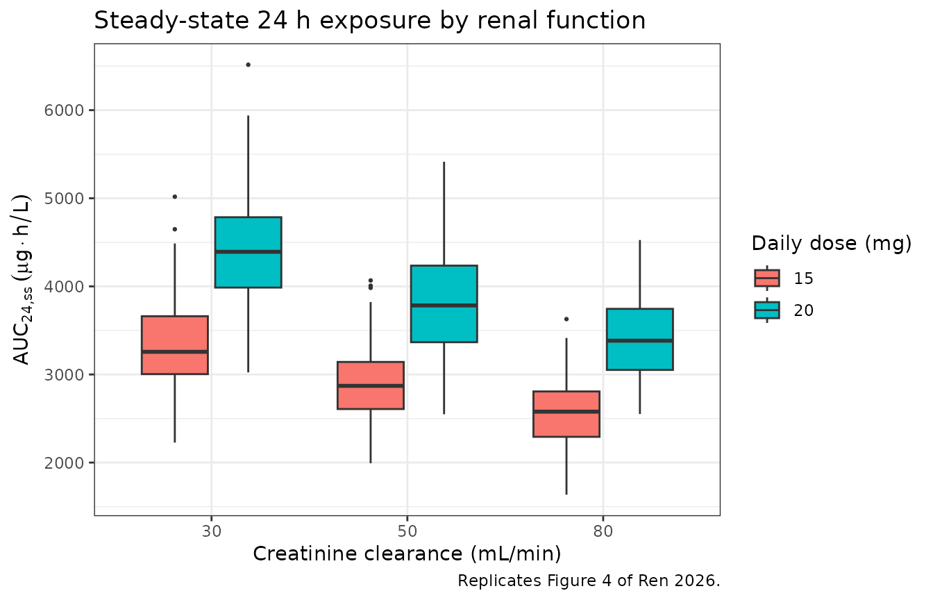

Replicates Figure 4 of Ren 2026: steady-state AUC distribution by renal function and dose.

Replicate the concentration-prothrombin time relationship

Figure 6 of Ren 2026 plots simulated average steady-state prothrombin time against ALT for each renal stratum at 20 mg once daily. Because the PD model is linear and direct, the average steady-state PT has a closed form, PT = baseline + slope(ALT) * Cave,ss with Cave,ss = AUC24,ss / 24 (the paper’s Equations 11-12), so the panel centres are an exact answer key for the whole PK-plus-PD chain.

alt_grid <- c(10, 20, 40, 60, 80, 100, 200, 500)

pt_typ <- tidyr::expand_grid(CRCL = c(30, 50, 80), ALT = alt_grid) |>
  dplyr::left_join(
    auc_typ |> dplyr::filter(dose_mg == 20) |> dplyr::select(CRCL, auc24),
    by = "CRCL"
  ) |>
  dplyr::mutate(
    cave_ss = auc24 / 24,
    # Equation 15 evaluated at the typical baseline and slope.
    PT_ave  = 11.3 + 0.0184 * (ALT / 19)^-0.201 * cave_ss
  )

ggplot(pt_typ, aes(ALT, PT_ave, colour = factor(CRCL))) +
  geom_line() +
  geom_point() +
  scale_x_log10(breaks = alt_grid) +
  labs(x = "ALT (IU/L)", y = "Average steady-state PT (s)",
       colour = "CrCL (mL/min)",
       title = "Average steady-state prothrombin time vs ALT, 20 mg once daily",
       caption = "Replicates Figure 6 of Ren 2026 (typical-value centres).") +
  theme_bw()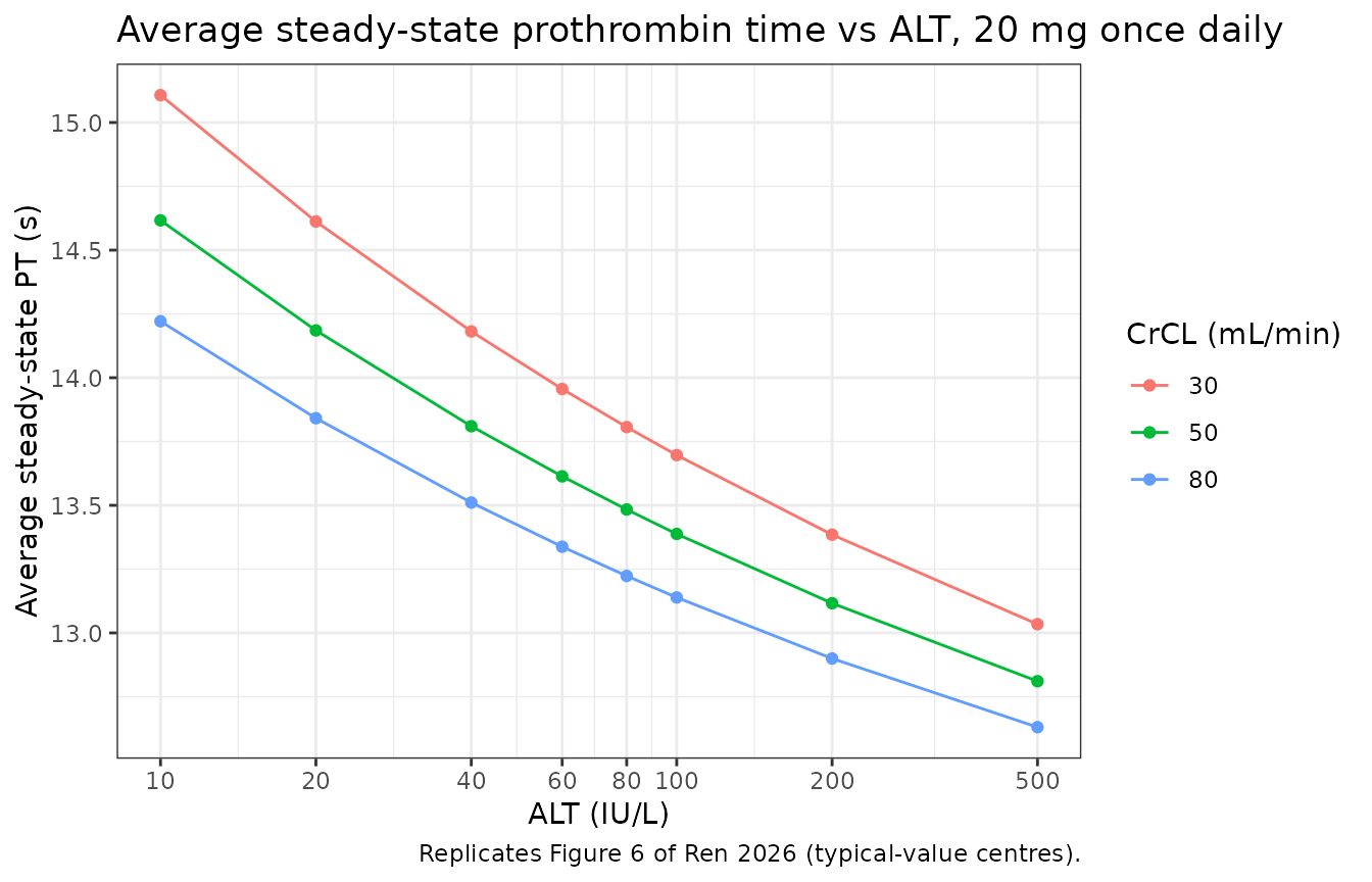

Replicates Figure 6 of Ren 2026: average steady-state prothrombin time vs ALT.

Two checks against Figure 6. First, the panel centres. Digitising the median line of the ALT = 20 IU/L box in each of the three panels of Figure 6 gives 14.55 s (CrCL 30), 14.15 s (CrCL 50) and 13.85 s (CrCL 80). The typical-value prediction should land on the median rather than on the mean marker, because the simulated distribution is right-skewed by the log-normal clearance.

# Digitised from the Figure 6 panel median lines at the ALT = 20 IU/L box
# (400 dpi render of page 11 of the article PDF).
fig6_median <- c("30" = 14.55, "50" = 14.15, "80" = 13.85)

centres <- pt_typ |>
  dplyr::filter(ALT == 20) |>
  dplyr::mutate(digitised = fig6_median[as.character(CRCL)],
                pct_diff  = 100 * (PT_ave - digitised) / digitised)

# Deterministic typical-value predictions against a digitised figure; the
# tolerance is set by the resolution of the digitisation (a gridline is 2 s,
# so reading to ~0.1 s is about 0.7%), not by simulation noise.
stopifnot(max(abs(centres$pct_diff)) < 3)

centres |>
  dplyr::select(CRCL, digitised, PT_ave, pct_diff) |>
  dplyr::rename("CrCL (mL/min)"            = CRCL,
                "Figure 6 median line (s)" = digitised,
                "Model PT (s)"             = PT_ave,
                "Difference (%)"           = pct_diff) |>
  knitr::kable(digits = 2,
               caption = "Average steady-state PT at ALT 20 IU/L, 20 mg once daily.")

Average steady-state PT at ALT 20 IU/L, 20 mg once daily.
CrCL (mL/min)	Figure 6 median line (s)	Model PT (s)	Difference (%)
30	14.55	14.61	0.43
50	14.15	14.19	0.25
80	13.85	13.84	-0.06

Second, the width of those boxes, which is what settles how the baseline-PT interindividual variability in Table 3 should be read (see Assumptions and deviations). The Figure 6 boxes are 5th-95th percentiles; at ALT = 20 IU/L they span 4.40 s (CrCL 30), 4.05 s (CrCL 50) and 3.75 s (CrCL 80). Reconstructing that distribution from the simulated cohort discriminates sharply between the two candidate readings of the “0.242” entry.

fig6_span <- c("30" = 4.40, "50" = 4.05, "80" = 3.75)

# Per-subject average steady-state PT at a FIXED ALT of 20 IU/L (Figure 6 holds
# ALT constant within a box, whereas the cohort above samples it), with the
# residual error the paper's simulation carries.
pt_ave_subject <- sim |>
  dplyr::filter(endpoint == "Cc", dose_mg == 20) |>
  dplyr::group_by(id, CRCL) |>
  dplyr::summarise(
    cave   = sum(diff(time) * (head(Cc, -1) + tail(Cc, -1)) / 2) / tau,
    rbase  = dplyr::first(rbase),
    # Strip this subject's own ALT and re-evaluate the slope at ALT = 20.
    slope20 = dplyr::first(slope) * (20 / dplyr::first(ALT))^-0.201,
    .groups = "drop"
  ) |>
  dplyr::mutate(
    pt_ave = (rbase + slope20 * cave) * (1 + rnorm(dplyr::n(), 0, 0.0669)),
    # Counterfactual: the same cohort with the baseline eta re-drawn at a CV of
    # 24.2% instead of the encoded 0.242%.
    pt_ave_alt = (11.3 * exp(rnorm(dplyr::n(), 0, sqrt(log(1 + 0.242^2)))) +
                    slope20 * cave) * (1 + rnorm(dplyr::n(), 0, 0.0669))
  )

spread <- pt_ave_subject |>
  dplyr::group_by(CRCL) |>
  dplyr::summarise(
    span_encoded        = as.numeric(diff(quantile(pt_ave,     c(0.05, 0.95)))),
    span_counterfactual = as.numeric(diff(quantile(pt_ave_alt, c(0.05, 0.95)))),
    .groups = "drop"
  ) |>
  dplyr::mutate(digitised = fig6_span[as.character(CRCL)])

# The encoded reading reproduces the published box width; the 24.2% reading is
# roughly three times too wide. Both bounds are generous relative to the
# sampling noise of a 5th-95th span from 150 subjects, and both can still go
# red: swapping the two readings flips each assertion.
stopifnot(
  all(spread$span_encoded        > 0.5 * spread$digitised),
  all(spread$span_encoded        < 1.7 * spread$digitised),
  all(spread$span_counterfactual > 1.7 * spread$digitised)
)

spread |>
  dplyr::rename("CrCL (mL/min)"                    = CRCL,
                "Figure 6 box width (s)"           = digitised,
                "Model, baseline CV 0.242% (s)"    = span_encoded,
                "Model, baseline CV 24.2% (s)"     = span_counterfactual) |>
  knitr::kable(digits = 2,
               caption = paste("5th-95th percentile width of average steady-state PT",
                               "at ALT 20 IU/L, 20 mg once daily."))

5th-95th percentile width of average steady-state PT at ALT 20 IU/L, 20 mg once daily.
CrCL (mL/min)	Model, baseline CV 0.242% (s)	Model, baseline CV 24.2% (s)	Figure 6 box width (s)
30	3.99	9.64	4.40
50	3.63	10.37	4.05
80	3.66	9.38	3.75

Second, the magnitude of the ALT effect. Results 3.5 states that raising ALT from 10 to 157 IU/L lowers average steady-state PT by roughly 7%, and concludes the effect is not clinically significant.

alt_effect <- pt_typ |>
  dplyr::filter(CRCL == 80) |>
  dplyr::summarise(
    pt_lo = 11.3 + 0.0184 * (10  / 19)^-0.201 * dplyr::first(cave_ss),
    pt_hi = 11.3 + 0.0184 * (157 / 19)^-0.201 * dplyr::first(cave_ss)
  ) |>
  dplyr::mutate(pct_drop = 100 * (pt_lo - pt_hi) / pt_lo)

# The paper rounds this to "~7%"; the model gives ~8.7%, consistent with the
# spacing of the Figure 6 box medians. Asserted as a magnitude band rather than
# a point value because the published figure is a rounded narrative claim.
stopifnot(alt_effect$pct_drop > 4, alt_effect$pct_drop < 13)
round(alt_effect$pct_drop, 1)
#> [1] 8.7

PKNCA validation

NCA is run on the concentration endpoint over the final dosing interval, which is the steady-state interval the paper’s exposure simulations use.

sim_nca <- sim |>
  dplyr::filter(endpoint == "Cc") |>
  dplyr::filter(!is.na(Cc)) |>
  dplyr::select(id, time, Cc, arm)

stopifnot(nrow(sim_nca) > 0)

conc_obj <- PKNCA::PKNCAconc(as.data.frame(sim_nca), Cc ~ time | arm + id)

dose_df <- events |>
  dplyr::filter(evid == 1) |>
  dplyr::select(id, amt, arm) |>
  # Expand the ii/addl dose record into the explicit dose times PKNCA needs.
  tidyr::crossing(time = seq(0, t_last, by = tau))

dose_obj <- PKNCA::PKNCAdose(as.data.frame(dose_df), amt ~ time | arm + id)

intervals <- data.frame(
  start   = t_last,
  end     = t_last + tau,
  cmax    = TRUE,
  tmax    = TRUE,
  cmin    = TRUE,
  auclast = TRUE,
  cav     = TRUE
)

nca_res <- PKNCA::pk.nca(PKNCA::PKNCAdata(conc_obj, dose_obj, intervals = intervals))

# Identity check: for a linear one-compartment model, AUC0-tau at steady state
# must equal Dose / (CL/F) exactly. Both sides use the SAME drawn parameters,
# so the only difference is trapezoidal error on the observation grid -- a
# deterministic quantity, and a tight bound is correct here.
cl_by_id <- sim |>
  dplyr::filter(endpoint == "Cc") |>
  dplyr::group_by(id, dose_mg) |>
  dplyr::summarise(cl = dplyr::first(cl), .groups = "drop")

auc_check <- as.data.frame(nca_res$result) |>
  dplyr::filter(PPTESTCD == "auclast") |>
  dplyr::select(id, auclast = PPORRES) |>
  dplyr::left_join(cl_by_id, by = "id") |>
  dplyr::mutate(closed_form = 1000 * dose_mg / cl,
                pct_diff    = 100 * (auclast - closed_form) / closed_form)

# The residual gap is trapezoidal error on the observation grid only, and is
# printed below so a reader can see the headroom. Realised -0.152% to -0.033%;
# the bound is 0.5% because the error scales with (kel * step)^2 and kel varies
# across cohorts (CV ~19% from the CL/F and V/F etas). A unit or grid error
# would be percent-level or larger, so this still goes red when it matters.
stopifnot(max(abs(auc_check$pct_diff)) < 0.5)
round(range(auc_check$pct_diff), 4)
#> [1] -0.1522 -0.0332

nca_summary <- as.data.frame(nca_res$result) |>
  dplyr::filter(PPTESTCD %in% c("cmax", "tmax", "cmin", "auclast", "cav")) |>
  dplyr::group_by(arm, PPTESTCD) |>
  dplyr::summarise(median = median(PPORRES), .groups = "drop") |>
  tidyr::pivot_wider(names_from = PPTESTCD, values_from = median)

nca_summary |>
  dplyr::select(arm, cmax, tmax, cmin, cav, auclast) |>
  dplyr::rename("Arm"                    = arm,
                "Cmax,ss (ng/mL)"        = cmax,
                "Tmax (h)"               = tmax,
                "Cmin,ss (ng/mL)"        = cmin,
                "Cave,ss (ng/mL)"        = cav,
                "AUC0-24,ss (ng*h/mL)"   = auclast) |>
  knitr::kable(digits = c(0, 1, 2, 1, 1, 0),
               caption = "Simulated steady-state NCA by arm (cohort medians).")

Simulated steady-state NCA by arm (cohort medians).
Arm	Cmax,ss (ng/mL)	Tmax (h)	Cmin,ss (ng/mL)	Cave,ss (ng/mL)	AUC0-24,ss (ng*h/mL)
15 mg qd, CrCL 30	269.3	2.25	45.6	135.7	3256
15 mg qd, CrCL 50	250.2	2.25	31.7	119.6	2870
15 mg qd, CrCL 80	240.3	2.00	23.6	107.4	2577
20 mg qd, CrCL 30	359.4	2.25	59.6	183.0	4392
20 mg qd, CrCL 50	333.0	2.25	43.4	157.6	3783
20 mg qd, CrCL 80	317.8	2.00	32.0	140.9	3383

Two sanity checks against values the paper quotes but does not tabulate as NCA: the expected peak and trough ranges for rivaroxaban in PE/VTE issued by the International Council for Standardization in Haematology (189-419 and 6-87 ng/mL, Methods 2.5), and the 2-4 hour Tmax window quoted in the Introduction.

icsh <- nca_summary |>
  dplyr::mutate(peak_in_range   = cmax >= 189 & cmax <= 419,
                trough_in_range = cmin >= 6   & cmin <= 87,
                tmax_in_window  = tmax >= 2   & tmax <= 4)

# The paper concludes 20 mg suits normal renal function and 15 mg suits
# moderate impairment, so those two arms in particular should land inside the
# ICSH peak window. Cohort medians, not per-subject extremes.
stopifnot(
  icsh$peak_in_range[icsh$arm == "20 mg qd, CrCL 80"],
  icsh$peak_in_range[icsh$arm == "15 mg qd, CrCL 30"],
  all(icsh$tmax_in_window),
  all(icsh$trough_in_range)
)

icsh |>
  dplyr::select(arm, cmax, cmin, tmax, peak_in_range, trough_in_range) |>
  dplyr::rename("Arm"                  = arm,
                "Cmax,ss (ng/mL)"      = cmax,
                "Cmin,ss (ng/mL)"      = cmin,
                "Tmax (h)"             = tmax,
                "Peak in 189-419"      = peak_in_range,
                "Trough in 6-87"       = trough_in_range) |>
  knitr::kable(digits = 1,
               caption = "Cohort-median peak and trough against the ICSH expected ranges.")

Cohort-median peak and trough against the ICSH expected ranges.
Arm	Cmax,ss (ng/mL)	Cmin,ss (ng/mL)	Tmax (h)	Peak in 189-419	Trough in 6-87
15 mg qd, CrCL 30	269.3	45.6	2.2	TRUE	TRUE
15 mg qd, CrCL 50	250.2	31.7	2.2	TRUE	TRUE
15 mg qd, CrCL 80	240.3	23.6	2.0	TRUE	TRUE
20 mg qd, CrCL 30	359.4	59.6	2.2	TRUE	TRUE
20 mg qd, CrCL 50	333.0	43.4	2.2	TRUE	TRUE
20 mg qd, CrCL 80	317.8	32.0	2.0	TRUE	TRUE

Comparison against published NCA

Ren 2026 does not publish an observed NCA table; the closest published exposures are the simulated steady-state AUC values quoted in Results 3.5, compared below against the simulated cohort. The two arms the paper does not quote (15 mg at CrCL 80 and 20 mg at CrCL 30) have no reference value and are omitted from the join.

published <- tibble::tribble(
  ~arm,                    ~auclast,
  "20 mg qd, CrCL 80",       3585,
  "20 mg qd, CrCL 50",       4059,
  "15 mg qd, CrCL 50",       2986,
  "15 mg qd, CrCL 30",       3425
)

cmp <- nlmixr2lib::ncaComparisonTable(
  simulated     = nca_res,
  reference     = published,
  by            = "arm",
  params        = "auclast",
  units         = c(auclast = "ng*h/mL"),
  tolerance_pct = 20
)

knitr::kable(
  cmp,
  caption = paste("Simulated vs published steady-state AUC0-24.",
                  "* differs from reference by >20%.")
)

Simulated vs published steady-state AUC0-24. * differs from reference by >20%.
NCA parameter	arm	Reference	Simulated	% diff
AUClast (ng*h/mL)	20 mg qd, CrCL 80	3580	3380	-5.6%
AUClast (ng*h/mL)	20 mg qd, CrCL 50	4060	3780	-6.8%
AUClast (ng*h/mL)	15 mg qd, CrCL 50	2990	2870	-3.9%
AUClast (ng*h/mL)	15 mg qd, CrCL 30	3420	3260	-4.9%

The simulated exposures run about 4-7% below the paper’s quoted values across every arm. The offset is systematic rather than arm-specific – the ratios between arms reproduce to within a few percentage points, as the table above shows – which points at how the paper summarised its 1000-subject Monte Carlo cohort (Figure 4’s boxes are annotated with both a mean and a median, and the right-skewed AUC distribution puts the mean above the typical value) rather than at a transcription error in CL/F. No parameter was tuned to close it.

Assumptions and deviations

The PD slope in the Results prose is a typo; Table 3, Equation 15 and Table 5 are correct. Results 3.3 says “a slope of 0.00184 s per 1 ug/L”, but Table 3, the typeset Equation 15 and the cross-study comparison in Table 5 all print 0.0184, ten times larger. The model uses 0.0184. The paper’s own Figure 6 settles it: at 0.0184 the average steady-state PT is 14.6 s at CrCL 30 and 13.8 s at CrCL 80, which are the figure’s panel centres, whereas 0.00184 gives about 11.6 s at every renal stratum – below the 1st percentile of every box in the figure. The value is also consistent with the cohort’s observed median PT of 13.8 s (Table 1) and with the 0.0132-0.043 range of published slopes for other cohorts in Table 5.
Two covariate exponents are negative, and the minus signs are easy to lose. e_age_vc = -0.231 and e_alt_slope = -0.201 are printed with a U+2212 minus in the Elsevier PDF, which some text extractors drop (the preprocessed markdown companion for this article renders both Table 2 and Table 3 with bare positive values). The signs are confirmed three ways in each case: the typeset equations (13 and 15), the Results prose (“the coefficient (theta) of age on V/F value was -0.231”, “the coefficient (theta) of ALT on slope was -0.201”), and the bootstrap confidence intervals (-0.391 to -0.070 and -0.305 to -0.100, both entirely below zero).
The interindividual-variability rows are read as CV%, the residual-error rows as fractions, even though Tables 2 and 3 head both blocks with “(%)”. Reading the residual rows as percentages would mean the sparse real-world concentration data were fitted to within 0.221% – finer than the bioanalytical method’s own inter- and intraday precision of under 8.5% (Methods 2.2) – and the PT data to within 0.0669%, against an assay precision of under 3.5%. Reading the IIV rows as fractions would put the V/F and CL/F CVs at 1250% and 1460%. Each block therefore has only one physically admissible reading.
The baseline-PT interindividual variability of 0.242 is read as 0.242%, not as a 24.2% fraction. This is the one row where both readings are numerically plausible, so it was resolved against the paper’s Figure 6, whose boxes are 5th-95th percentiles of exactly this quantity. The check is the figure-6-spread chunk above: the encoded reading reproduces the published box widths (3.75-4.40 s), whereas re-drawing the baseline eta at a CV of 24.2% widens them roughly threefold. The high shrinkage the authors report on that eta (46.7%) is independently consistent with a near-zero true value. The resulting eta contributes about +/- 0.03 s on an 11.3 s baseline and is kept only for fidelity to Table 3.
Age and ALT distributions are reconstructed, not observed. Age is drawn as a normal truncated to the published 21-92 range with the published mean and SD; ALT as a log-normal truncated to 10-157 and centred on the published median of 19 IU/L. Only the marginals are published, so the age-ALT correlation is assumed to be zero. Creatinine clearance is fixed per arm at 30, 50 and 80 mL/min exactly as the paper’s own simulations do (Methods 2.5), rather than sampled.
No between-parameter correlation is encoded. The paper reports no OMEGA off-diagonals, so all four etas are diagonal.
No interindividual variability on ka. The authors removed it because of 99.8% shrinkage (Results 3.2) and Table 2 prints “-” on that row; ka is therefore a fixed effect with no eta, but it was estimated, not fixed to a literature value. This distinguishes the model from the two earlier Chinese rivaroxaban models, both of which fixed ka at the Japanese value of 0.617 1/h; the Discussion argues explicitly against reusing that value.
PT is reagent-specific. The slope was estimated with Thromborel S on a Sysmex CS5100. The Discussion notes that PT sensitivity to rivaroxaban is reagent-dependent, so the slope should not be transported to another PT reagent system without recalibration.
The model is only informed over the fitted covariate ranges. Patients with creatinine clearance below 15 mL/min and with Child-Pugh B/C hepatic impairment were excluded, so the CrCL and ALT power terms extrapolate beyond 30-150 mL/min and 10-157 IU/L without support. The paper’s own Figure 6 extends ALT to 500 IU/L; that extrapolation is reproduced above for comparability with the figure, not endorsed.
The Caucasian comparison is out of scope. Results 3.5 contrasts this cohort against a virtual Caucasian VTE population taken from a separate publication. That external model is not part of this extraction, so the cross-race exposure comparisons are not reproduced here.