Ranibizumab in preterm infants (Fidler 2020)
Source:vignettes/articles/Fidler_2020_ranibizumab.Rmd
Fidler_2020_ranibizumab.RmdModel and source
- Citation: Fidler M, Fleck BW, Stahl A, Marlow N, Chastain JE, Li J, Lepore D, Reynolds JD, Chiang MF, Fielder AR; RAINBOW study group. Ranibizumab population pharmacokinetics and free VEGF pharmacodynamics in preterm infants with retinopathy of prematurity in the RAINBOW trial. Transl Vis Sci Technol. 2020;9(8):43. doi:10.1167/tvst.9.8.43
- Description: One-compartment population PK model with first-order absorption for serum ranibizumab after bilateral intravitreal injection in preterm infants with retinopathy of prematurity (RAINBOW trial; Fidler et al. 2020, TVST). The vitreous acts as a first-order depot (Ka = ocular elimination rate, flip-flop kinetics) into a systemic central compartment. Typical values are expressed for a 70-kg adult and scaled to the infant by body weight (fixed allometric exponent 0.75 on CL/F, linear on V/F); CL/F also carries a fixed creatinine-clearance adjustment evaluated at the study-median infant CrCl (54.82 mL/min, modified Schwartz) relative to the adult median (65.22 mL/min) with the adult exponent 0.266. Correlated log-normal IIV on CL/F, V/F and Ka; log-normal residual error.
- Article: Transl Vis Sci Technol 2020;9(8):43
The paper also examined plasma free VEGF as a pharmacodynamic marker. Free VEGF did not differ between the laser and ranibizumab arms or over time, and individual predicted ranibizumab concentrations showed no relationship with observed free VEGF (Results, Figure 2, Supplementary Figure S6), so no PD model was developed and only the PK model is provided here.
Population
RAINBOW randomised 225 preterm infants with retinopathy of prematurity (ROP) 1:1:1 to a single bilateral intravitreal injection of ranibizumab 0.1 mg or 0.2 mg per eye, or to laser therapy, in 26 countries. Sparse serum samples were drawn in odd-numbered ranibizumab-treated infants at day 1, day 15 (days 7-21) and day 29 (days 22-28); 95 infants (45 at 0.1 mg, 50 at 0.2 mg) contributed serum concentrations (Table 1). Across the two ranibizumab arms (Table 1), mean gestational age at birth was 25.8-26.5 weeks, mean birth weight 791-886 g, mean postnatal age at treatment about 11 weeks and median weight at treatment 1.7-1.8 kg (range 0.8-3.9 kg); 46% were female, 59% Caucasian and 32% Asian.
#> List of 11
#>  $ species       : chr "human"
#>  $ n_subjects    : int 95
#>  $ n_studies     : int 1
#>  $ age_range     : chr "Preterm infants; postnatal age at baseline mean 10.8-11.1 weeks (SD 3.9-4.5) by arm; gestational age at birth m"| __truncated__
#>  $ weight_range  : chr "0.8-4.2 kg at baseline (median 1.7-1.8 kg by arm)"
#>  $ sex_female_pct: num 46.3
#>  $ race_ethnicity: Named num [1:4] 59.1 31.5 2.7 6.7
#>   ..- attr(*, "names")= chr [1:4] "Caucasian" "Asian" "Black" "Other"
#>  $ disease_state : chr "Retinopathy of prematurity (ROP) requiring treatment"
#>  $ dose_range    : chr "Single bilateral intravitreal injection of ranibizumab 0.1 mg or 0.2 mg per eye (0.2 or 0.4 mg total per infant"| __truncated__
#>  $ regions       : chr "26 countries; investigator sites (Supplementary Table S3) in the USA, Mexico, Japan, Taiwan, India, Malaysia, S"| __truncated__
#>  $ notes         : chr "RAINBOW trial. PK sampling in odd-numbered ranibizumab-treated infants at day 1, day 15 (7-21) and day 29 (22-2"| __truncated__
Source trace
| Equation / parameter | Value | Source location |
|---|---|---|
lcl (CL/F, 70-kg adult) |
log(28.48) L/day | Table 2 |
lvc (V/F, 70-kg adult) |
log(27.58) L | Table 2 |
lka (Ka) |
log(0.12) 1/day | Table 2 |
e_wt_cl |
fixed 0.75 | Supplementary Appendix, CL equation (w/70)^(3/4)
|
e_wt_vc |
fixed 1 | Supplementary Appendix, V equation (w/70)
|
e_crcl_cl |
fixed 0.266 | Supplementary Appendix, “thetaCRCL = 0.266” (adult value) |
| Infant CrCl 54.82 mL/min, adult CrCl 65.22 mL/min | constants | Supplementary Appendix (MCRCL, MCRCLa) |
etalcl variance |
log(1 + 0.3492^2) = 0.11506 | Table 2, BSV 34.92% CV |
etalvc variance |
log(1 + 2.9056^2) = 2.24522 | Table 2, BSV 290.56% CV |
etalka variance |
log(1 + 0.1628^2) = 0.026159 | Table 2, BSV 16.28% CV |
| cov(CL, V) | 0.491 x sqrt(0.11506 x 2.24522) = 0.24956 | Supplementary Table S1, step 3 correlation 0.491 |
| cov(V, Ka) | -0.55 x sqrt(2.24522 x 0.026159) = -0.13329 | Supplementary Table S1, step 5 correlation -0.55 |
| cov(CL, Ka) | 0 | Supplementary Table S1 step 6 not selected; Appendix “with the exception of … omegaKa and omegaCl” |
expSd |
0.60 | Table 2, “Lognormal SD” |
| One compartment, first-order absorption from the eye | structure | Final Model: Description |
Cc ~ lnorm(expSd) |
log-normal residual | Base Model; Final Model: Description |
Virtual cohort and simulation
Weight at treatment is drawn log-normally around the reported median
of 1.8 kg and restricted to the reported range 0.8-4.2 kg by redrawing
(not clamping) out-of-range values. The dose is the total amount
injected into both eyes (0.2 mg for the 0.1 mg/eye arm, 0.4 mg for the
0.2 mg/eye arm); the single vitreous compartment pools both
eyes.
rxode2::rxSetSeed(20200729)
n_per_arm <- 200
draw_wt <- function(n) {
  wt <- numeric(0)
  while (length(wt) < n) {
    x <- exp(rnorm(n, log(1.8), 0.35))
    wt <- c(wt, x[x >= 0.8 & x <= 4.2])
  }
  wt[seq_len(n)]
}

arms <- data.frame(
  treatment = c("0.1 mg/eye", "0.2 mg/eye"),
  amt = c(0.2, 0.4)
)
cohort <- arms[rep(1:2, each = n_per_arm), ]
cohort$id <- seq_len(nrow(cohort))
cohort$WT <- draw_wt(nrow(cohort))

obs_times <- sort(unique(c(0, 10^seq(-2, log10(90), length.out = 120))))

dose_rows <- cohort |>
  mutate(time = 0, evid = 1, cmt = "vitreous")
obs_rows <- cohort |>
  select(id, treatment, WT) |>
  tidyr::crossing(time = obs_times) |>
  mutate(amt = 0, evid = 0, cmt = "central")
events <- bind_rows(dose_rows, obs_rows) |>
  arrange(id, time, desc(evid)) |>
  as.data.frame()

mod <- readModelDb("Fidler_2020_ranibizumab")
sim <- rxode2::rxSolve(mod, events, keep = c("treatment", "WT"),
                       returnType = "data.frame")
#> ℹ parameter labels from comments will be replaced by 'label()'
Typical-value check against the closed form
For a typical 1.8 kg infant the model solution must equal the analytic one-compartment first-order-absorption profile, and the Supplementary Appendix secondary-parameter equations give Tmax, Cmax and AUCinf directly. Both sides use the same parameters, so the tolerance is numerical only.
mod_typ <- rxode2::zeroRe(mod)
#> ℹ parameter labels from comments will be replaced by 'label()'
ev_typ <- rxode2::et(amt = 0.4, cmt = "vitreous") |>
  rxode2::et(obs_times, cmt = "central")
typ <- rxode2::rxSolve(mod_typ, ev_typ, params = c(WT = 1.8),
                       returnType = "data.frame")
#> ℹ omega/sigma items treated as zero: 'etalka', 'etalvc', 'etalcl'

cl_typ <- 28.48 * (1.8 / 70)^0.75 * (54.82 / 65.22)^0.266
v_typ <- 27.58 * (1.8 / 70)
ka_typ <- 0.12
kel_typ <- cl_typ / v_typ
closed <- function(t, dose) {
  dose * ka_typ / (v_typ * (ka_typ - kel_typ)) *
    (exp(-kel_typ * t) - exp(-ka_typ * t)) * 1000
}
stopifnot(max(abs(typ$Cc - closed(typ$time, 0.4))) < 1e-3 * max(typ$Cc))

tmax_typ <- log(ka_typ / kel_typ) / (ka_typ - kel_typ)
data.frame(
  quantity = c("CL/F (L/day)", "V/F (L)", "Ka half-life (day)",
               "Kel half-life (day)", "Tmax (day)",
               "Cmax 0.4 mg (ng/mL)", "AUCinf 0.4 mg (ng*day/mL)"),
  typical_1.8kg = c(cl_typ, v_typ, log(2) / ka_typ, log(2) / kel_typ,
                    tmax_typ, max(closed(seq(0, 10, by = 0.001), 0.4)),
                    0.4 / cl_typ * 1000),
  Table3_median_0.2mg_arm = c(1.7, 0.7, 5.6, 0.3, 1.3, 24.3, 232.0)
) |>
  knitr::kable(digits = 2,
caption = "Typical 1.8 kg infant versus the Table 3 post hoc medians (0.2 mg/eye arm).")| quantity | typical_1.8kg | Table3_median_0.2mg_arm |
|---|---|---|
| CL/F (L/day) | 1.75 | 1.7 |
| V/F (L) | 0.71 | 0.7 |
| Ka half-life (day) | 5.78 | 5.6 |
| Kel half-life (day) | 0.28 | 0.3 |
| Tmax (day) | 1.29 | 1.3 |
| Cmax 0.4 mg (ng/mL) | 23.55 | 24.3 |
| AUCinf 0.4 mg (ng*day/mL) | 229.06 | 232.0 |
The typical infant reproduces every Table 3 median: the ocular (absorption) half-life of about 5.6-5.8 days is the apparent serum half-life (flip-flop), and serum elimination proper has a half-life of about 0.3 days.
Replicate Figure 1 (simulated prediction interval)
sim |>
  filter(time > 0) |>
  group_by(treatment, time) |>
  summarise(med = median(Cc), lo = quantile(Cc, 0.05),
            hi = quantile(Cc, 0.95), .groups = "drop") |>
  ggplot(aes(time, med)) +
  geom_ribbon(aes(ymin = lo, ymax = hi), alpha = 0.25) +
  geom_line() +
  facet_wrap(~treatment) +
  scale_y_log10() +
  coord_cartesian(xlim = c(0, 30), ylim = c(0.01, 200)) +
  labs(x = "Time after injection (day)", y = "Serum ranibizumab (ng/mL)",
       caption = "Median and 90% interval of 200 simulated infants per arm; replicates the layout of Figure 1 of Fidler 2020.")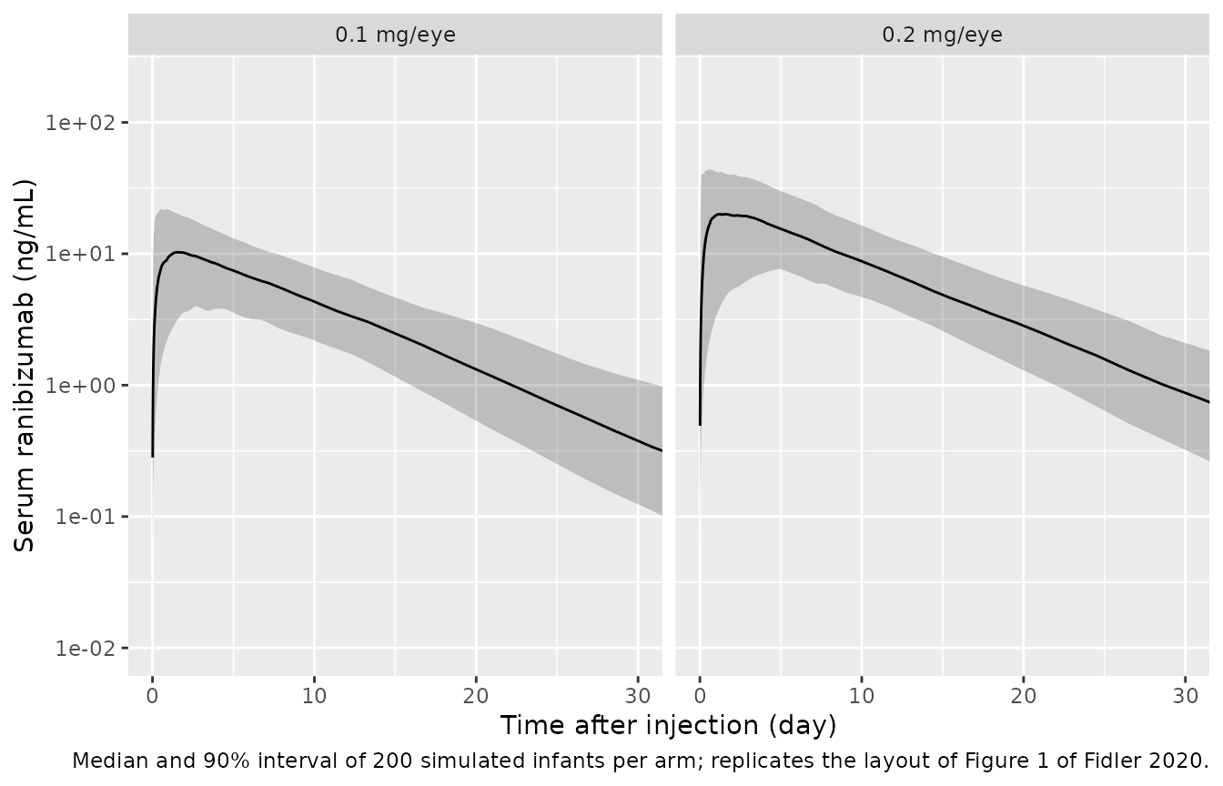
PKNCA validation
conc_df <- sim |>
  filter(!is.na(Cc)) |>
  select(id, time, Cc, treatment)
dose_df <- events |>
  filter(evid == 1) |>
  select(id, time, amt, treatment)

conc_obj <- PKNCA::PKNCAconc(conc_df, Cc ~ time | treatment + id,
                             concu = "ng/mL", timeu = "day")
#> Warning in assert_conc(conc, any_missing_conc = any_missing_conc): Negative
#> concentrations found
dose_obj <- PKNCA::PKNCAdose(dose_df, amt ~ time | treatment + id,
                             doseu = "mg")
intervals <- data.frame(start = 0, end = Inf, cmax = TRUE, tmax = TRUE,
                        aucinf.obs = TRUE)
nca_res <- PKNCA::pk.nca(PKNCA::PKNCAdata(conc_obj, dose_obj,
                                          intervals = intervals))
#> Warning in assert_conc(conc = conc): Negative concentrations found
#> Warning in assert_conc(conc = conc): Negative concentrations found
#> Warning in assert_conc(conc = conc): Negative concentrations found
#> Warning in assert_conc(conc = conc): Negative concentrations found
#> Warning in assert_conc(conc = conc): Negative concentrations found
#> Warning in assert_conc(conc = conc): Negative concentrations found
#> Warning in log(data$conc): NaNs produced
#> Warning in assert_conc(conc, any_missing_conc = any_missing_conc): Negative
#> concentrations found
#> Warning in log(conc.2/conc.1): NaNs produced
nca_df <- as.data.frame(nca_res)

sim_med <- nca_df |>
  filter(PPTESTCD %in% c("cmax", "tmax", "aucinf.obs")) |>
  group_by(treatment, PPTESTCD) |>
  summarise(PPORRES = median(PPORRES, na.rm = TRUE), .groups = "drop")
Comparison against Fidler 2020 Table 3 (post hoc medians)
published <- data.frame(
  treatment = c("0.1 mg/eye", "0.2 mg/eye"),
  cmax = c(11.5, 24.3),
  tmax = c(1.3, 1.3),
  aucinf.obs = c(113.6, 232.0)
)
cmp <- nlmixr2lib::ncaComparisonTable(
  simulated = sim_med,
  reference = published,
  by = "treatment",
  units = c(cmax = "ng/mL", tmax = "day", aucinf.obs = "day*ng/mL"),
  tolerance_pct = 20
)
knitr::kable(cmp, caption = "Simulated median NCA vs. Fidler 2020 Table 3 medians. * differs by >20%.")| NCA parameter | treatment | Reference | Simulated | % diff |
|---|---|---|---|---|
| Cmax (ng/mL) | 0.1 mg/eye | 11.5 | 11 | -4.2% |
| Cmax (ng/mL) | 0.2 mg/eye | 24.3 | 21 | -13.8% |
| Tmax (day) | 0.1 mg/eye | 1.3 | 1.34 | +3.0% |
| Tmax (day) | 0.2 mg/eye | 1.3 | 1.56 | +20.0% |
| AUC0-∞ (obs) (day*ng/mL) | 0.1 mg/eye | 114 | 109 | -4.5% |
| AUC0-∞ (obs) (day*ng/mL) | 0.2 mg/eye | 232 | 227 | -2.3% |
# Structural gates on the cohort centre. A mis-scaled dose (per eye vs both
# eyes), a wrong allometric reference or a unit slip moves these medians by
# 50-100%, far outside the 20% envelope.
med <- tidyr::pivot_wider(sim_med, names_from = PPTESTCD, values_from = PPORRES) |>
  left_join(published, by = "treatment", suffix = c("_sim", "_pub"))
stopifnot(
  all(abs(med$aucinf.obs_sim / med$aucinf.obs_pub - 1) < 0.2),
  all(abs(med$cmax_sim / med$cmax_pub - 1) < 0.25)
)

# Mass balance with each subject's own clearance: AUCinf * CL/F == dose.
indiv <- sim |>
  group_by(id) |>
  summarise(cl = first(cl), .groups = "drop")
mb <- nca_df |>
  filter(PPTESTCD == "aucinf.obs") |>
  inner_join(indiv, by = "id") |>
  inner_join(dose_df, by = c("id", "treatment")) |>
  mutate(ratio = PPORRES * cl / (amt * 1000))
stopifnot(abs(median(mb$ratio, na.rm = TRUE) - 1) < 0.02)
Cmax and AUCinf are dose proportional across the arms, as reported, and the cohort medians match the Table 3 post hoc medians. Simulated median Tmax is somewhat later than the Table 3 median: infants drawn with a large V/F (the V/F variability is 290% CV) have a slower serum elimination and so a later peak, whereas the Table 3 values are post hoc estimates from sparse data and are shrunk towards the typical value (typical Tmax 1.29 days).
Assumptions and deviations
- Creatinine-clearance term is a constant. The paper evaluates the adult creatinine-clearance effect at the study-median infant CrCl (54.82 mL/min, modified Schwartz) for every infant, because site-measured serum creatinine was unreliable (23.3% of values below 0.01 mg/dL). The model therefore has no CrCl covariate; the factor (54.82/65.22)^0.266 = 0.955 multiplies CL/F for everyone.
- Final-model IIV correlations. Table 2 reports only the variances. The two retained covariances are taken from the correlations printed in Supplementary Table S1 when each was added: 0.491 for CL/F-V/F (step 3) and -0.55 for Ka-V/F (step 5, the final model). The step-3 value may have shifted slightly in the later steps; this affects only the joint spread of the simulated parameters.
- Ka rounding. Table 2 prints Ka as 0.12 1/day (95% CI 0.12-0.13), giving a typical ocular half-life of 5.8 days versus the 5.6-day post hoc median in Table 3; the printed value is used unchanged.
- Adult starting values in the Supplementary Appendix. The appendix quotes CLa = 23.8 L/day and Va = 2.97 L from the prior adult model; the re-estimated Table 2 values (28.48 L/day, 27.58 L) are the final estimates and reproduce the Table 3 infant medians, so they are used.
- Bilateral dosing. The total dose to both eyes enters one pooled vitreous compartment. The Supplementary Appendix Cmax/AUCinf equations with the total dose reproduce the Table 3 medians, confirming this reading.
- Weight distribution. Only the median and range are published; a log-normal with SD 0.35 on the log scale truncated to 0.8-4.2 kg is assumed.
- Table 3 medians are post hoc estimates from sparse data and are shrunk towards the typical value, so their spread (not shown) is narrower than a fully stochastic simulation; only medians are compared.