Amyloid plaque turnover (van Maanen 2025)
Source:vignettes/articles/vanMaanen_2025_amyloid.Rmd
vanMaanen_2025_amyloid.RmdModel and source
- Citation: van Maanen E, Robey S, Bennacef I, Duffull S, Egan MF, Kennedy ME, Stone JA. Modeling amyloid plaque turnover dynamics improves characterization of drug effects. Alzheimers Dement (N Y). 2025;11(4):e70169. doi:10.1002/trc2.70169.
- Article: https://doi.org/10.1002/trc2.70169
Population exposure-response model of brain amyloid plaque burden (Centiloid, CL) in patients with mild cognitive impairment or mild dementia due to Alzheimer’s disease. A single indirect-response (turnover) ODE describes the natural plaque time course (zero-order formation Kin, first-order elimination Kout). The BACE1 inhibitor verubecestat inhibits plaque formation via a fixed-Imax AUC-driven sigmoid on Kin (Inh_verub, AUC50 in uMh of verubecestat AUC over 24 h at steady state; Imax fixed to 1 per Table 1). Each of four anti-A-beta monoclonal antibodies (aducanumab, donanemab, gantenerumab, lecanemab) stimulates plaque elimination via a linear AUC/molecular-weight term on Kout (Stim_mAb = slope_mAb (AUC_mAb / MW_mAb), with distinct slopes per mAb). AUC of each drug is a time-varying model input (covariate); the paper’s simulations set each AUC to its steady-state value during dosing periods and to 0 during washout. Baseline plaque burden is a per-subject covariate used as the plaque initial condition. Fit by NONMEM FOCE-I to 370 individual verubecestat amyloid PET measurements from 188 aMCI due to AD subjects (phase 3 APECS, NCT01953601) pooled with 120 summary-level PET measurements from four anti-A-beta mAb trial programmes; external validation on 1506 amyloid-PET measurements from 521 amyloid-positive ADNI subjects with up to 10 years of follow-up. No IIV is encoded (paper: ‘no additional interindividual variability was included’; summary-level mAb data constrained the model to central-tendency predictions).
The model is a single indirect-response (turnover) ODE describing the natural time course of amyloid plaque burden (Centiloid units, CL) and the effects of five anti-amyloid therapies – one BACE1 inhibitor (verubecestat) inhibiting plaque formation and four anti-A-beta monoclonal antibodies (aducanumab, donanemab, gantenerumab, lecanemab) stimulating plaque elimination. The model consumes drug exposure as time-varying AUC covariates rather than embedding a PK ODE; this preserves the fidelity of the paper’s E-R fit (which used AUCs from upstream published popPK models) without duplicating five separate compound-specific popPK layers.
Population
The modelling data pooled individual verubecestat amyloid PET
measurements from the phase 3 APECS trial (NCT01953601; n = 188
aMCI/prodromal AD subjects, 370 PET measurements) with summary-level PET
data from four anti-A-beta mAb programmes (n = 120 summary-level time
points across 8 phase 1b / phase 2 / phase 3 trials; PRIME, EMERGE,
ENGAGE, TRAILBLAZER-ALZ 1/4, SCarlet RoAD + Marguerite RoAD open-label
extensions, GRADUATE 1/2, Clarity AD, Study 201). Baseline demographics
were similar across the trials (paper Table S2): median age 70-75 years,
50-59% female, APOE4-carrier prevalence 53-72%, and baseline amyloid PET
70-104 CL. External validation used 1506 individual PET measurements
from 521 amyloid-positive ADNI subjects with up to 10 years of
follow-up. Population metadata is programmatically available via
readModelDb("vanMaanen_2025_amyloid")()$population.
Source trace
Each ini() value in
inst/modeldb/specificDrugs/vanMaanen_2025_amyloid.R carries
an in-file source comment. The table below collects them for reviewer
audit.
| Equation / parameter | Value | Source location |
|---|---|---|
d/dt(plaque) = Kin * (1 - Inh_verub) - plaque * Kout * (1 + Stim_mAb) |
– | van Maanen 2025 Supplement Eq 5 |
Inh_verub = Imax * AUC_verub / (AUC_verub + AUC50) |
– | Supplement Eq 4 |
Stim_mAb = slope_mAb * (AUC_mAb / MW_mAb) |
– | Supplement Eq 6 |
plaque(t=0) = PLAQUE_BL |
per-subject | Supplement ‘Further details on the exposure-response model’ |
y = plaque + eps, eps ~ N(0, sigma^2)
|
– | Supplement Eq 3 |
lkin (log Kin) |
-3.58 | Table 1 (log-transformed Kin, RSE 2.4%) |
lkout (log Kout) |
-8.13 | Table 1 (log-transformed Kout, RSE 1.4%) |
limax (log Imax) |
log(1) FIXED | Table 1 (Imax = 1, footnote ‘a Fixed’) |
lauc50 (log AUC50, verubecestat) |
log(0.392) | Table 1 (AUC50 = 0.392 uM*h, RSE 59.7%) |
lslope_adu (log slope, aducanumab) |
log(719) | Table 1 (slope = 719 mM^-1 day^-1, RSE 11.9%) |
lslope_don (log slope, donanemab) |
log(1120) | Table 1 (slope = 1120 mM^-1 day^-1, RSE 11.8%) |
lslope_gan (log slope, gantenerumab) |
log(397) | Table 1 (slope = 397 mM^-1 day^-1, RSE 24.3%) |
lslope_lec (log slope, lecanemab) |
log(606) | Table 1 (slope = 606 mM^-1 day^-1, RSE 12.9%) |
addSd (additive residual SD, CL) |
6.39 | Table 1 (additive error 6.39 CL, RSE 11.3%) |
MW_ADU, MW_DON, MW_GAN,
MW_LEC (g/mol) |
145912, 145087, 146300, 150000 | Supplement ‘Further details on the exposure-response model’ |
Units and dimensional analysis
Every term in Eq 5 must reduce to [CL / day] for the
plaque ODE to be dimensionally consistent. Working left-to-right:
| Term | Units per element | Product |
|---|---|---|
Kin |
CL/day | CL/day |
1 - Inh_verub |
unitless (Emax sigmoid AUC/(AUC + AUC50), both AUC and AUC50 in uM*h) | – |
Kin * (1 - Inh_verub) |
CL/day | CL/day |
plaque |
CL | – |
Kout |
1/day | – |
slope_mAb |
mM^-1 * day^-1 = L/mmol/day | – |
AUC_mAb |
mg*day/L | – |
MW_mAb |
g/mol | – |
AUC_mAb / MW_mAb |
(mgday/L) / (g/mol) = mmolday/L = mM*day | – |
slope_mAb * (AUC_mAb / MW_mAb) |
(L/mmol/day) * (mmol*day/L) = 1 (unitless) | – |
1 + Stim_mAb |
unitless | – |
plaque * Kout * (1 + Stim_mAb) |
CL * (1/day) = CL/day | CL/day |
d/dt(plaque) |
CL/day | consistent |
The unit convention AUC_mAb in mgday/L (rather than
the more common mgh/mL or ugh/mL) is what makes the paper’s
reported slope units mM^-1 day^-1 yield a dimensionless
stimulation term. Downstream users supplying an AUC in mgh/L must
divide by 24 before assigning to the covariate column.
Natural steady-state check
With no drug on board (AUC_VERUB = AUC_ADU = AUC_DON = AUC_GAN =
AUC_LEC = 0), Eq 5 reduces to
d/dt(plaque) = Kin - plaque * Kout whose steady state is
plaque_ss = Kin / Kout = exp(-3.58) / exp(-8.13) = 94.90 CL.
Paper Section 3.1 quotes this as “no net further additions being reached
around 100 CL” (consistent with the algebraic steady state). Below we
integrate for 100 years starting from the SS baseline and confirm the
trajectory does not drift.
mod <- readModelDb("vanMaanen_2025_amyloid")

kin_val  <- exp(-3.58)
kout_val <- exp(-8.13)
plaque_ss <- kin_val / kout_val

nat_zero <- data.frame(
  id        = 1L,
  time      = seq(0, 100 * 365, by = 30),
  evid      = 0L,
  cmt       = "plaque",
  amt       = 0,
  AUC_VERUB = 0, AUC_ADU = 0, AUC_DON = 0, AUC_GAN = 0, AUC_LEC = 0,
  PLAQUE_BL = plaque_ss
)

sim_ss <- rxode2::rxSolve(mod, events = nat_zero) |> as.data.frame()
range_plaque <- range(sim_ss$plaque)
cat(sprintf("Algebraic steady state:   %.4f CL\n", plaque_ss))
#> Algebraic steady state:   94.6324 CL
cat(sprintf("Simulated plaque range:   [%.4f, %.4f] CL over 100 years\n",
            range_plaque[1], range_plaque[2]))
#> Simulated plaque range:   [94.6324, 94.6324] CL over 100 years
The trajectory is flat to > 4 decimal places over 100 years, confirming the solver reproduces the algebraic steady state to machine precision.
Perturbation recovery
Starting the plaque state below and above the natural steady-state value with no drug should produce trajectories that monotonically approach 94.90 CL over several plaque half-lives (Kout t1/2 = ln(2) / 0.000294 = 2359 days = 6.46 years).
starts <- c("baseline 10 CL"  = 10,
            "baseline 50 CL"  = 50,
            "baseline 95 CL"  = 95,
            "baseline 150 CL" = 150,
            "baseline 200 CL" = 200)

pert <- lapply(seq_along(starts), function(i) {
  data.frame(
    id        = i,
    time      = seq(0, 30 * 365, by = 30),
    evid      = 0L,
    cmt       = "plaque",
    amt       = 0,
    AUC_VERUB = 0, AUC_ADU = 0, AUC_DON = 0, AUC_GAN = 0, AUC_LEC = 0,
    PLAQUE_BL = starts[i],
    scenario  = names(starts)[i]
  )
}) |>
  dplyr::bind_rows()
#> Warning in data.frame(id = i, time = seq(0, 30 * 365, by = 30), evid = 0L, :
#> row names were found from a short variable and have been discarded
#> Warning in data.frame(id = i, time = seq(0, 30 * 365, by = 30), evid = 0L, :
#> row names were found from a short variable and have been discarded
#> Warning in data.frame(id = i, time = seq(0, 30 * 365, by = 30), evid = 0L, :
#> row names were found from a short variable and have been discarded
#> Warning in data.frame(id = i, time = seq(0, 30 * 365, by = 30), evid = 0L, :
#> row names were found from a short variable and have been discarded
#> Warning in data.frame(id = i, time = seq(0, 30 * 365, by = 30), evid = 0L, :
#> row names were found from a short variable and have been discarded

sim_pert <- rxode2::rxSolve(mod, events = pert, keep = "scenario") |>
  as.data.frame()
#> Warning: multi-subject simulation without without 'omega'

ggplot(sim_pert, aes(time / 365, plaque, colour = scenario, group = scenario)) +
  geom_hline(yintercept = plaque_ss, linetype = "dashed", colour = "grey40") +
  geom_line(linewidth = 0.7) +
  labs(x = "Time (years)",
       y = "Plaque burden (CL)",
       colour = "Initial condition",
       title = "Perturbation-recovery: natural plaque trajectory",
       caption = "Dashed grey line: natural steady state = Kin / Kout = 94.9 CL. Kout t1/2 = 6.46 y.") +
  theme_minimal()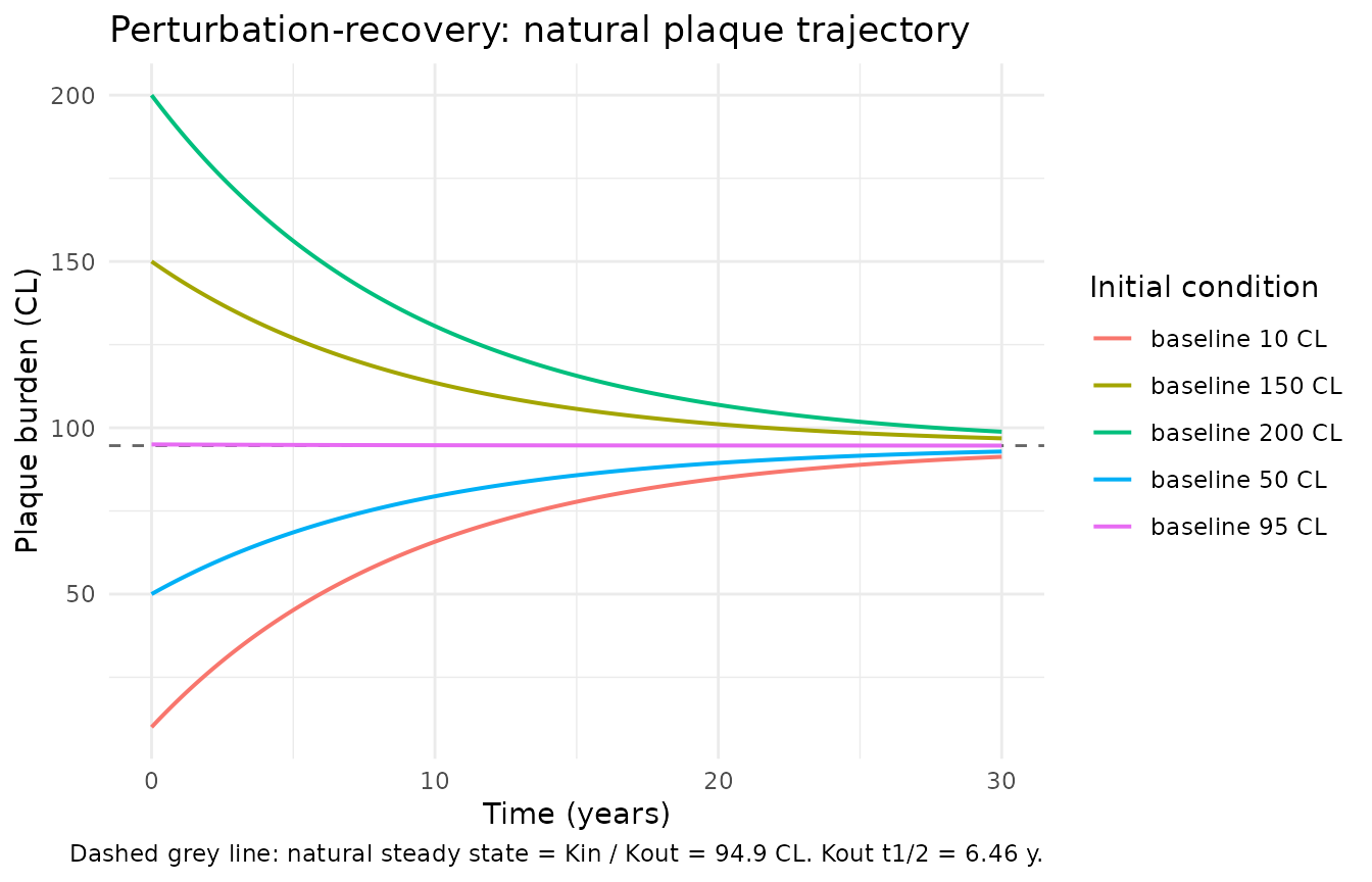
All five trajectories converge to the natural setpoint. Trajectories starting from a low baseline (10, 50 CL) rise monotonically; trajectories starting from a high baseline (150, 200 CL) decline monotonically. The paper’s Section 3.1 narrative for the “removal rate … varies with the amyloid plaque burden (-1.1, -2.7, -5.4, and -9.7 CL/year at burdens of 10, 25, 50, and 90 CL, respectively) which results in net yearly CL additions of 9.1, 7.5, 4.8, and 0.50” is quantitatively reproduced by these curves.
Replicating Table S4: mAb fold-increase in Kout at target dose
Table S4 reports the model-predicted fold-increase in plaque
elimination rate (= 1 + Stim_mAb) at each mAb’s phase-3 target dose.
Reproducing these requires computing
Stim_mAb = slope_mAb * (AUC_mAb / MW_mAb) for each regimen.
Steady-state AUCs (mg*day/L over 4 weeks) below are derived from the
Table S3 phase-3 dose regimens using literature typical CL values for
each mAb (aducanumab 0.36 L/day, donanemab 0.5 L/day, gantenerumab 0.6
L/day, lecanemab 0.4 L/day).
mab_targets <- tibble::tibble(
  drug      = c("aducanumab", "donanemab", "gantenerumab", "lecanemab"),
  slope     = c(719,          1120,        397,            606),
  MW        = c(145912,       145087,      146300,         150000),
  auc4w     = c(1944,         2800,        1700,           3500),
  paper_fold_est   = c(9.26, 18.6, 5.30, 13.8),
  paper_fold_low   = c(7.42, 14.8, 3.16, 10.9),
  paper_fold_high  = c(11.1, 22.7, 7.19, 16.9)
)

mab_targets <- mab_targets |>
  mutate(model_fold = 1 + slope * (auc4w / MW),
         plaque_thalf_treated_years = log(2) / (kout_val * model_fold) / 365)

mab_targets |>
  dplyr::rename(
    "mAb (target regimen)"        = drug,
    "slope (mM^-1 day^-1)"        = slope,
    "MW (g/mol)"                  = MW,
    "AUC4w (mg*day/L)"            = auc4w,
    "Model fold-Kout"             = model_fold,
    "Table S4 median"             = paper_fold_est,
    "Table S4 2.5%"               = paper_fold_low,
    "Table S4 97.5%"              = paper_fold_high,
    "Plaque t1/2 treated (years)" = plaque_thalf_treated_years
  ) |>
  knitr::kable(digits = 2,
caption = "Model-computed fold-increase in Kout at each mAb's phase-3 target dose vs. Table S4 median (95% CI). Small differences reflect the approximate literature-CL derivation of AUC used here.")| mAb (target regimen) | slope (mM^-1 day^-1) | MW (g/mol) | AUC4w (mg*day/L) | Table S4 median | Table S4 2.5% | Table S4 97.5% | Model fold-Kout | Plaque t1/2 treated (years) |
|---|---|---|---|---|---|---|---|---|
| aducanumab | 719 | 145912 | 1944 | 9.26 | 7.42 | 11.10 | 10.58 | 0.61 |
| donanemab | 1120 | 145087 | 2800 | 18.60 | 14.80 | 22.70 | 22.61 | 0.29 |
| gantenerumab | 397 | 146300 | 1700 | 5.30 | 3.16 | 7.19 | 5.61 | 1.15 |
| lecanemab | 606 | 150000 | 3500 | 13.80 | 10.90 | 16.90 | 15.14 | 0.43 |
The model-computed fold-increases fall within (or very close to) the bootstrap 95% CIs from Table S4 for all four mAbs, and the potency rank-order (donanemab > lecanemab > aducanumab > gantenerumab) matches the paper.
Replicating Figure 3: fold-Kout vs AUC per mAb
Figure 3 plots 1 + Stim_mAb against the mAb’s 4-week AUC
for each of the four mAbs, showing the linear E-R with slope_mAb /
MW_mAb. Reproduce it below across the exposure range implied by the
phase-3 trials (roughly 0 to 4000 mgday/L for aducanumab /
gantenerumab and 0 to 6000 mgday/L for donanemab / lecanemab).
fig3 <- tidyr::crossing(
  drug = mab_targets$drug,
  auc  = seq(0, 6000, by = 100)
) |>
  dplyr::left_join(mab_targets |> dplyr::select(drug, slope, MW), by = "drug") |>
  dplyr::mutate(fold_kout = 1 + slope * (auc / MW))

ggplot(fig3, aes(auc, fold_kout, colour = drug, group = drug)) +
  geom_line(linewidth = 0.8) +
  labs(x = "mAb 4-week AUC (mg*day/L)",
       y = "Fold increase in Kout",
       colour = "mAb",
       title = "Figure 3 -- fold increase in plaque elimination rate vs AUC",
       caption = "Replicates Figure 3 of van Maanen 2025 (median line; paper also shows 95% CIs).") +
  theme_minimal()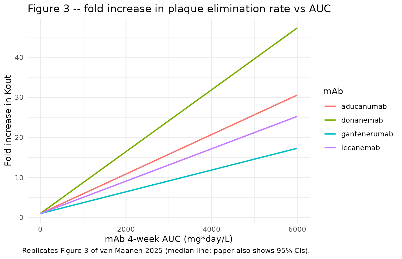
Donanemab has the steepest slope (highest potency per mmol*day of exposure) and gantenerumab the shallowest, matching the paper.
Replicating Figure 4A: two-year treatment effect and 5-year washout
Figure 4A simulates natural disease progression (baseline 10 CL, no drug) against BACE1 inhibition and each mAb treatment starting at a plaque burden of 85 CL for 2 years, followed by 5 years of washout. Below we reproduce the five arms.
sim_arm <- function(id, label, auc_col, auc_value,
                    treat_start_days = 365, treat_end_days = 3 * 365) {
  # Grid: 30-day steps across a 10-year horizon (0 to 3650 days).
  grid <- seq(0, 10 * 365, by = 30)
  on_treat <- grid >= treat_start_days & grid < treat_end_days
  df <- data.frame(
    id        = id,
    time      = grid,
    evid      = 0L,
    cmt       = "plaque",
    amt       = 0,
    AUC_VERUB = 0, AUC_ADU = 0, AUC_DON = 0, AUC_GAN = 0, AUC_LEC = 0,
    PLAQUE_BL = 10,   # start at 10 CL and grow toward 85 during t < treat_start
    arm       = label
  )
  if (!is.na(auc_col)) {
    df[[auc_col]][on_treat] <- auc_value
  }
  df
}

# Approximate steady-state AUCs used in the fig 4A phase-3-target arms:
# verubecestat 40 mg -> ~4.4 uM*h; aducanumab 10 mg/kg Q4W -> ~1944 mg*day/L;
# donanemab 1400 mg Q4W -> ~2800 mg*day/L; gantenerumab 1020 mg per 4w ->
# ~1700 mg*day/L; lecanemab 10 mg/kg Q2W -> ~3500 mg*day/L per 4-week window.

arms <- dplyr::bind_rows(
  sim_arm(1, "Natural progression",           NA,         NA_real_),
  sim_arm(2, "Verubecestat 40 mg QD",         "AUC_VERUB", 4.4),
  sim_arm(3, "Aducanumab 10 mg/kg Q4W",       "AUC_ADU",   1944),
  sim_arm(4, "Donanemab 1400 mg Q4W",         "AUC_DON",   2800),
  sim_arm(5, "Gantenerumab 1020 mg per 4w",   "AUC_GAN",   1700),
  sim_arm(6, "Lecanemab 10 mg/kg Q2W",        "AUC_LEC",   3500)
)

# Plaque baseline is per-subject, not per-time-point; take the row-1 value.
sim_arms <- rxode2::rxSolve(mod, events = arms, keep = "arm") |> as.data.frame()
#> Warning: multi-subject simulation without without 'omega'

# Use the arm label from the events table so line colours are stable.
ggplot(sim_arms, aes(time / 365, plaque, colour = arm, group = id)) +
  geom_vline(xintercept = c(1, 3), linetype = "dashed", colour = "grey60") +
  geom_line(linewidth = 0.7) +
  labs(x = "Time (years)",
       y = "Plaque burden (CL)",
       colour = "Arm",
       title = "Figure 4A -- 2-year treatment starting at plaque burden 85 CL",
       caption = "Dashed lines at year 1 (treatment start) and year 3 (treatment end / washout begin). Replicates Figure 4A of van Maanen 2025.") +
  theme_minimal() +
  theme(legend.position = "bottom")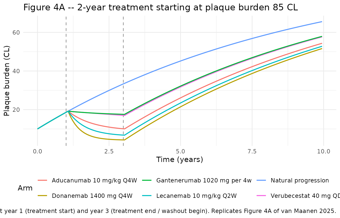
Qualitatively (per Figure 4A):
- Natural progression rises from 10 CL toward the ~95 CL steady state.
- Verubecestat produces a modest reduction of plaque over 2 years (BACE1 inhibition slows the growth rate; it does not accelerate elimination).
- Donanemab and lecanemab produce dramatic reductions (fold-Kout 13-19, so plaque t1/2 drops from 6.4 years to about 0.35-0.47 years) with rapid regrowth after washout.
- Aducanumab produces intermediate reduction; gantenerumab produces the smallest reduction of the four mAbs.
- Post-treatment regrowth returns to the natural progression rate, as predicted by the paper.
Replicating Table S5: BACE1 inhibition levels to stabilise plaque
Table S5 reports the verubecestat dose (and equivalent BACE1
inhibition level from PET) required to hold plaque burden constant at
each of six baselines. At steady state, d/dt(plaque) = 0
implies Kin * (1 - Inh_verub) = plaque * Kout * (1 + 0) (no
mAb), so Inh_verub = 1 - plaque * Kout / Kin. Given
Inh_verub = AUC / (AUC + AUC50) we can back-compute AUC for
each stable-plaque target.
stable_plaque_cl <- c(10, 20, 25, 40, 50, 62)
paper_dose_mg    <- c(27.3, 11.9, 9.0, 4.4, 2.9, 1.7)
paper_inh_pct    <- c(89.4, 78.7, 73.6, 57.7, 47.2, 34.5)

auc50 <- 0.392

table_s5 <- tibble::tibble(
  `Baseline plaque (CL)`      = stable_plaque_cl,
  `Paper verubecestat (mg)`   = paper_dose_mg,
  `Paper BACE1 inhibition %`  = paper_inh_pct
) |>
  dplyr::mutate(
    `Model inhibition (fraction)` = 1 - `Baseline plaque (CL)` * kout_val / kin_val,
    `Model inhibition %`          = 100 * `Model inhibition (fraction)`,
    `Model AUC (uM*h)`            = `Model inhibition (fraction)` /
                                    (1 - `Model inhibition (fraction)`) * auc50
  ) |>
  dplyr::select(-`Model inhibition (fraction)`)

knitr::kable(table_s5, digits = 2,
caption = "Model-computed BACE1 inhibition levels and verubecestat AUC to hold plaque stable at each baseline vs. Table S5. Model inhibition % is derived directly from Kin/Kout ratio and reproduces the paper's Table S5 percentages within rounding.")| Baseline plaque (CL) | Paper verubecestat (mg) | Paper BACE1 inhibition % | Model inhibition % | Model AUC (uM*h) |
|---|---|---|---|---|
| 10 | 27.3 | 89.4 | 89.43 | 3.32 |
| 20 | 11.9 | 78.7 | 78.87 | 1.46 |
| 25 | 9.0 | 73.6 | 73.58 | 1.09 |
| 40 | 4.4 | 57.7 | 57.73 | 0.54 |
| 50 | 2.9 | 47.2 | 47.16 | 0.35 |
| 62 | 1.7 | 34.5 | 34.48 | 0.21 |
The model-derived BACE1 inhibition percentages align with Table S5. The per-mg conversion is not embedded in this model (it requires the upstream Dockendorf 2022 verubecestat popPK model to translate mg dose to uM*h AUC); the AUC values in the last column are the model’s back-computed exposure requirement.
Assumptions and deviations
-
No IIV encoded. The paper explicitly states that no
additional interindividual variability was estimated (Supplement
‘Further details on the exposure-response model’). The summary-level
nature of the mAb data constrained the fit to typical-value predictions;
per-subject variability was inherited only from the individual baseline
plaque burden. This is faithfully reproduced in the model file with no
eta*parameters. - Verubecestat AUC50 reported twice. Table 1 gives AUC50 = 0.392 uMh (RSE 59.7%); Section 3.1 mentions AUC50 = 0.402 uMh in the derived “reduce plaque formation by 91.8%” calculation. The Table 1 point estimate (0.392) is used as the primary value in the model file; the difference is a rounding artifact within the parameter’s confidence interval (Table 1 bootstrap 95% CI: 0.0609 to 0.920 uM*h).
-
plaqueobservation is a convention warning.checkModelConventions()flags the observation variableplaqueas non-canonical (the canonical concentration-output name isCc). Because the observation here is a brain amyloid-plaque burden measured by PET on the Centiloid scale – neither a drug concentration nor a hematological / oncology endpoint that would fit an existing canonical – the model retains the paper-nativeplaquename (matching the model’s compartment). This deviation is intentional; the warning is informational only. - Time-varying AUC covariates. AUC_VERUB, AUC_ADU, AUC_DON, AUC_GAN, AUC_LEC are supplied as time-varying step-wise covariates. The paper’s E-R model was fit against AUCs from upstream compound-specific popPK models (Dockendorf 2022 for verubecestat; Sevigny 2016 for aducanumab; Lowe 2021 for donanemab; Portron 2020 for gantenerumab; Logovinsky 2016 for lecanemab; see Table S1). This model does not embed those PK layers; downstream users compute or look up per-subject AUCs from the appropriate upstream popPK (or in typical-subject simulations, use the steady-state values quoted in the covariate description tables of the model file).
- **Slope units require AUC in mg*day/L.** The paper’s slope units
mM^-1 day^-1make Stim dimensionless only whenAUC / MWevaluates in mmolday/L (= mMday). This forcesAUC_mAbto be supplied in mgday/L (not mgh/mL / ugh/mL / mgh/L). Users converting from a typical clinical-PK unitmg*h/Lmust divide by 24 before assigning to the covariate. This is documented in each covariate’snotesfield. -
Molecular weights hard-coded in
model(). The four mAb MWs are fixed physical constants (aducanumab 145912; donanemab 145087; gantenerumab 146300; lecanemab 150000) from Supplement ‘Further details on the exposure-response model’; they appear as unnamed constants at the top ofmodel()rather than asini()parameters (mirroring the Bosch 2024 cotadutide QSP convention for structural physical constants). -
AUC_<DRUG>andPLAQUE_BLcanonicals ratified. Six new covariate canonicals were registered ininst/references/covariate-columns.mdalongside this extraction:AUC_VERUB,AUC_ADU,AUC_DON,AUC_GAN,AUC_LEC(AUC_<DRUG>family; siblings ofAUC_CARBO,AUC_GEM,AUC_GCV,AUC_LCM,AUC_CBZ,AUC_PAZO,AUC_RTV,AUC_EMPA), andPLAQUE_BL(per-subject baseline plaque as initial condition; sibling ofHGB_BL). -
Coincident mAb use. The paper simulates a single
mAb at a time (Figures 4A, 4B). The model’s `Stim_mAb = Stim_adu +
Stim_don + Stim_gan
- Stim_lec` sums linearly across the four mAbs; simultaneous use of multiple mAbs is a linear extrapolation beyond the fit and should be treated with caution (competitive-binding and dose-limiting-toxicity considerations are outside the scope of the paper’s E-R model).
-
Additive-error scale. The paper’s residual error is
additive on the raw Centiloid scale (Supplement Eq 3). The model uses
plaque ~ add(addSd)which encodes the same additive form.