Generic monoclonal antibody population PK (van den Berg 2025)
Source:vignettes/articles/vandenBerg_2025_genericMab.Rmd
vandenBerg_2025_genericMab.RmdModel and source
- Article: mAbs 2025;17(1):2512217
- Supplement: Supplementary Sections M1-M5, Figures S1-S7 and Table S1
(
KMAB_A_2512217_SM8525.docx), plus the full 160-model dataset (KMAB_A_2512217_SM8524.xlsx), both published with the open-access article (PMC12128664).
This paper is a systematic meta-analysis of 160 published two-compartment population PK models covering 69 marketed canonical IgG monoclonal antibodies. Rather than cataloguing those models only, the authors build an original deliverable from them: a generic mAb model whose every parameter is the across-model median, which they simulate in NONMEM 7.5.0 to show that “one model” produces plausible IgG kinetics. That generic model, and the two weight-covariate configurations the authors simulate alongside it, are what this vignette validates.
Three model files come out of the paper:
mods <- list(
  generic  = rxode2::rxode(readModelDb("vandenBerg_2025_genericMab_mbma")),
  combI    = rxode2::rxode(readModelDb("vandenBerg_2025_genericMab_allometricClVc_mbma")),
  combII   = rxode2::rxode(readModelDb("vandenBerg_2025_genericMab_allometricAll_mbma"))
)
#> ℹ parameter labels from comments will be replaced by 'label()'
tibble::tibble(
  Model = names(mods),
  `nlmixr2lib name` = c(
    "vandenBerg_2025_genericMab_mbma",
    "vandenBerg_2025_genericMab_allometricClVc_mbma",
    "vandenBerg_2025_genericMab_allometricAll_mbma"
  ),
  Role = c(
    "Generic mAb model: depot + 2 compartments, IIV on CL/Vc/ka, no covariates (Figure 5c,d; Suppl. M5)",
    "Covariate combination I: body weight on CL and Vc only (Figure 4h; Suppl. Figure S7)",
    "Covariate combination II: body weight on CL, Vc, Vp and Q (Figure 4h; Suppl. Figure S7)"
  )
) |>
knitr::kable(caption = "Models contributed by van den Berg 2025.")| Model | nlmixr2lib name | Role |
|---|---|---|
| generic | vandenBerg_2025_genericMab_mbma | Generic mAb model: depot + 2 compartments, IIV on CL/Vc/ka, no covariates (Figure 5c,d; Suppl. M5) |
| combI | vandenBerg_2025_genericMab_allometricClVc_mbma | Covariate combination I: body weight on CL and Vc only (Figure 4h; Suppl. Figure S7) |
| combII | vandenBerg_2025_genericMab_allometricAll_mbma | Covariate combination II: body weight on CL, Vc, Vp and Q (Figure 4h; Suppl. Figure S7) |
- Citation: van den Berg SPH, Adolfsen PEA, Dorlo TPC, Rispens T. Does one model fit all mAbs? An evaluation of population pharmacokinetic models. mAbs. 2025;17(1):2512217. doi:10.1080/19420862.2025.2512217
Population
The “population” behind this model is not a trial cohort but a body of literature. IMGT/mAb-DB was queried for marketed canonical IgG monoclonal antibodies, PubMed was searched per mAb, and 303 candidate population PK models were filtered down to 160 models of 69 mAbs by excluding one-compartment models, paediatric-only models, subcutaneous models that fixed bioavailability to 100%, models without a linear clearance component, models fixing more than two of CL/Vc/Vp/Q, PBPK and non-population models, non-i.v./s.c. routes, FcRn-engineered mAbs, and models with insufficient reporting (Figure 1a, Methods “PK models acquisition”).
Those 160 models were fitted to a summed 143,094
patients across the 157 models that reported a patient count
(Supplementary Table S1 column N); patients are
double-counted wherever several models were fitted to overlapping
datasets, so that figure is an upper bound rather than a cohort size.
The median (IQR) model used 5250 (1788; 10223) samples, i.e. 8.6 (5.7;
13.3) samples per patient (Results “Sample size matters”).
By model (Table 1): IgG1 71.9%, IgG2 8.8%, IgG4 18.1%, IgG2/4 1.2%; chimeric 20.0%, humanised 35.0%, fully human 45.0%; i.v. only 67.5%, s.c. only 0.6%, i.v./s.c. 31.9%. Nonlinear elimination was present in 47.5% of models and time-dependent clearance in 19.4% – neither is carried into the generic model, which is deliberately a linear-clearance description of IgG homeostasis.
The same information is available programmatically:
str(mods$generic$population, max.level = 1)
#> List of 12
#>  $ species          : chr "human"
#>  $ n_subjects       : int 143094
#>  $ n_studies        : int 160
#>  $ n_models         : int 160
#>  $ n_mabs           : int 69
#>  $ disease_state    : chr "Mixed. The pooled evidence base spans every indication in which a marketed canonical IgG mAb has had a populati"| __truncated__
#>  $ dose_range       : chr "Not summarised across the source models. The paper's illustrative simulation used a single 100 mg intravenous o"| __truncated__
#>  $ regions          : chr "Global; the collected models were not stratified by region."
#>  $ design           : chr "Meta-analysis of published population PK model PARAMETER ESTIMATES, not of raw or digitised concentration data."| __truncated__
#>  $ reference_subject: chr "A typical individual with no covariates. Parameter estimates were pooled AS REPORTED, without normalisation to "| __truncated__
#>  $ composition      : chr "By model (n = 160): IgG1 71.9%, IgG2 8.8%, IgG4 18.1%, IgG2/4 1.2%; chimeric 20.0%, humanised 35.0%, fully huma"| __truncated__
#>  $ notes            : chr "n_subjects is the SUM of the per-model patient counts across the 157 of 160 models that reported one (Supplemen"| __truncated__
Source trace
Every ini() entry carries an in-file comment pointing at
its source location. The table below collects them.
| Equation / parameter | Value | Source location |
|---|---|---|
lcl (CL) |
0.22 L/day | Figure 5c caption; Suppl. M5 $THETA 0.22 FIX; Results
median (IQR) 0.22 (0.17; 0.29) |
lvc (Vc) |
3.42 L | Figure 5c caption; Suppl. M5 $THETA 3.42 FIX; Results
median (IQR) 3.42 (2.96; 3.99) |
lvp (Vp) |
2.68 L | Figure 5c caption; Suppl. M5 $THETA 2.68 FIX; Results
median (IQR) 2.68 (2.09; 3.54) |
lq (Q) |
0.54 L/day | Figure 5c caption; Suppl. M5 $THETA 0.54 FIX; Results
median (IQR) 0.54 (0.36; 0.84) |
lka (ka) |
0.25 /day | Figure 5c caption; Suppl. M5
$THETA 0.25 FIX ; T_ka (/d); Results median (IQR) 0.25
(0.18; 0.29) |
lfdepot (F) |
0.69 | Figure 5c caption; Suppl. M5 $THETA 0.69 FIX and
F1 = THETA(6); Results median (IQR) 69 (61; 77)% |
etalcl |
var 0.097 (31.9 CV%) | Figure 5c caption; Suppl. M5 $OMEGA 0.097 FIX ; IIV_CL;
Figure 3a |
etalvc |
var 0.056 (24 CV%) | Figure 5c caption; Suppl. M5 $OMEGA 0.056 FIX ; IIV_V1;
Figure 3a |
etalka |
var 0.26 (54.8 CV%) | Figure 5c caption; Suppl. M5
$OMEGA 0.26 FIX ; IIV_ka
|
propSd (generic) |
1e-5 | Suppl. M5 $THETA 0.00001 FIX ; T_Prop_RE (sd) with
$SIGMA 1 FIX; Methods: “No RUV or covariates were
introduced” |
e_wt_cl, e_wt_vc (combination I) |
0.69, 0.67 | Suppl. Figure S7 caption: “I) CL_WT = 0.69, Vc_WT = 0.67” |
e_wt_cl, e_wt_vc, e_wt_vp,
e_wt_q (combination II) |
0.75, 0.85, 0.85, 0.77 | Suppl. Figure S7 caption: “II) CL_WT = 0.75, Vc_WT = 0.85, Vp_WT = 0.85, Q_WT = 0.77” |
| Reference weight 70 kg | 70 kg | Suppl. Figure S7 caption worked example
CL40kg = 0.22 x (40/70)^0.75; Results median (IQR)
reference weight 70 (69; 75) kg |
d/dt(depot), d/dt(central),
d/dt(peripheral1)
|
n/a | Suppl. M5 $DES (DEPOT /
CENTRAL / PERI), with
K20 = CL/VC, K23 = Q/VC,
K32 = Q/VP
|
f(depot) <- exp(lfdepot) |
n/a | Suppl. M5 $PK, F1 = THETA(6)
|
Cc <- central / vc |
n/a | Suppl. M5 $PK, S2 = VC
|
| Terminal half-life formula | n/a | Suppl. Section M4 (Toutain and Bousquet-Melou 2004) |
The published medians reproduce from the deposited dataset
The paper deposits the full 160-model dataset (Supplementary Table
S1). The structural medians quoted in the Results and in the Figure 5
caption reproduce from it exactly – CL 0.2200, Vc 3.4230, Vp 2.6800, Q
0.5390 over all 160 models, and ka 0.2485, F 0.6945 over the 52 models
built on both i.v. and s.c. data – along with every interquartile range.
That check was run once at extraction time against
KMAB_A_2512217_SM8524.xlsx; it is recorded here rather than
re-run in the vignette because the spreadsheet is not redistributed with
this package.
Part 1 – the generic model
Virtual cohort
The paper simulated 500 virtual individuals given a single 100 mg dose by either route. This vignette uses 200 per arm, which is the cohort cap for validation vignettes and is ample to characterise the median and the 5th/95th percentiles.
set.seed(20250521)

n_per_arm <- 200L
obs_times <- sort(unique(c(
  seq(0, 14, by = 0.5), seq(15, 60, by = 1), seq(62, 168, by = 2)
)))

make_arm <- function(n, arm, dose_cmt, id_offset) {
  subj <- tibble::tibble(id = id_offset + seq_len(n), treatment = arm)
  doses <- subj |>
    mutate(time = 0, amt = 100, evid = 1L, cmt = dose_cmt)
  obs <- subj |>
    tidyr::crossing(time = obs_times) |>
    mutate(amt = NA_real_, evid = 0L, cmt = "central")
  bind_rows(doses, obs) |>
    arrange(id, time, desc(evid))
}

events <- bind_rows(
  make_arm(n_per_arm, "100 mg IV", "central", 0L),
  make_arm(n_per_arm, "100 mg SC", "depot",   n_per_arm)
)

stopifnot(!anyDuplicated(events[events$evid == 0L, c("id", "time")]))
Observation rows point at the ODE state central;
Cc is an algebraic observable and is returned as a column
regardless.
Simulation
sim <- rxode2::rxSolve(
  mods$generic, events = events, keep = "treatment", useLinCmt = FALSE
) |>
  as.data.frame()

stopifnot(dplyr::n_distinct(sim$id) == 2L * n_per_arm)
Replicating Figure 5c and 5d
Figure 5c and 5d of van den Berg 2025 overlay the generic model’s median and 5th/95th percentiles on the typical-value profiles of the individual published i.v. (5c) and s.c. (5d) models. The published models are not redistributable, so only the generic-model envelope is reproduced here.
# Replicates Figure 5c (IV) and 5d (SC) of van den Berg 2025: median and
# 5th/95th percentile concentration-time profile of the generic model after a
# single 100 mg dose.
# rxSolve returns observation records only -- there is no evid column in its output.
sim |>
  group_by(treatment, time) |>
  summarise(
    Q05 = quantile(Cc, 0.05),
    Q50 = quantile(Cc, 0.50),
    Q95 = quantile(Cc, 0.95),
    .groups = "drop"
  ) |>
  ggplot(aes(time, Q50)) +
  geom_ribbon(aes(ymin = Q05, ymax = Q95), alpha = 0.25) +
  geom_line(linewidth = 0.8) +
  facet_wrap(~treatment) +
  scale_y_log10() +
  labs(
    x = "Time (days)", y = "Serum concentration (mg/L)",
    title = "Generic mAb model, single 100 mg dose",
    caption = "Replicates Figures 5c and 5d of van den Berg 2025 (generic-model envelope only)."
  ) +
  theme_bw()
#> Warning in scale_y_log10(): log-10 transformation introduced infinite values.
#> log-10 transformation introduced infinite values.
#> log-10 transformation introduced infinite values.
#> log-10 transformation introduced infinite values.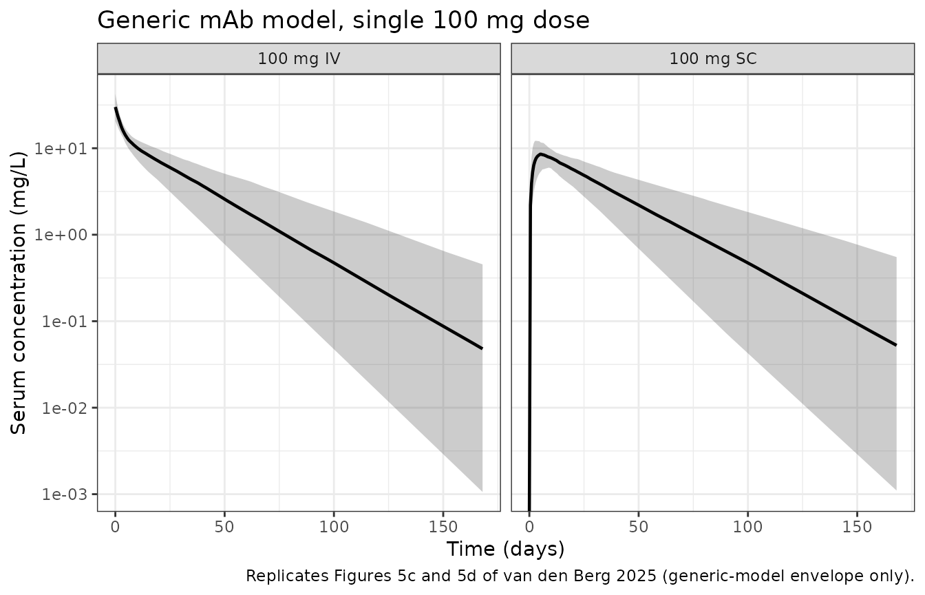
Terminal half-life – the paper’s headline number
The paper reports a terminal half-life of 21.3 days for the generic model, with 5th and 95th percentiles of 13.4 and 35.5 days (Results “Generic model”). Half-life is computed here with the paper’s own formula from Supplementary Section M4,
t1/2 = ln(2) / beta where
2*beta = (k12 + k21 + k10) - sqrt((k12 + k21 + k10)^2 - 4*k21*k10),
applied to each simulated individual’s own CL, Vc, Vp and Q.
terminal_half_life <- function(cl, vc, vp, q) {
  k10 <- cl / vc
  k12 <- q / vc
  k21 <- q / vp
  s <- k12 + k21 + k10
  log(2) / ((s - sqrt(s^2 - 4 * k21 * k10)) / 2)
}

thalf <- sim |>
  filter(treatment == "100 mg IV") |>
  distinct(id, cl, vc, vp, q) |>
  mutate(t_half = terminal_half_life(cl, vc, vp, q))

thalf_summary <- tibble::tibble(
  Quantity = c("Median", "5th percentile", "95th percentile"),
  Simulated = c(
    median(thalf$t_half),
    quantile(thalf$t_half, 0.05),
    quantile(thalf$t_half, 0.95)
  ),
  Published = c(21.3, 13.4, 35.5)
) |>
  mutate(`% diff` = (Simulated - Published) / Published * 100)

knitr::kable(
  thalf_summary,
  digits = 2,
  caption = "Terminal half-life (days) of the generic model, 200 virtual individuals, versus the 500-individual values reported in van den Berg 2025 Results 'Generic model'."
)| Quantity | Simulated | Published | % diff |
|---|---|---|---|
| Median | 20.53 | 21.3 | -3.63 |
| 5th percentile | 12.41 | 13.4 | -7.42 |
| 95th percentile | 34.12 | 35.5 | -3.89 |
# Agreement within 10% is expected: the paper drew a different (larger) random
# sample, so the residue is Monte-Carlo noise, not a structural discrepancy.
stopifnot(all(abs(thalf_summary$`% diff`) < 10))
The typical-value (no-IIV) half-life is a pure function of the four fixed disposition parameters and should land next to the simulated median:
typ <- as.data.frame(rxode2::rxSolve(
  rxode2::zeroRe(mods$generic),
  events = filter(events, treatment == "100 mg IV", id == 1),
  useLinCmt = FALSE
))
#> ℹ omega/sigma items treated as zero: 'etalcl', 'etalvc', 'etalka'
cat(sprintf(
  "Typical-value terminal half-life: %.2f days\n",
  terminal_half_life(typ$cl[1], typ$vc[1], typ$vp[1], typ$q[1])
))
#> Typical-value terminal half-life: 20.88 days
Structural identities
Two identities must hold exactly for a linear two-compartment model given an i.v. bolus, and both are checked per subject rather than on a median (a median carries sampling noise; the per-subject identity does not):
Cmax = Dose / VcAUC0-inf = Dose / CL
and, comparing arms of the same individual model,
F = AUC_SC / AUC_IV = 0.69.
iv <- sim |> filter(treatment == "100 mg IV")

cmax_check <- iv |>
  group_by(id) |>
  summarise(cmax = max(Cc), predicted = 100 / first(vc), .groups = "drop") |>
  mutate(rel = cmax / predicted - 1)

stopifnot(max(abs(cmax_check$rel)) < 1e-6)
cat(sprintf(
  "Cmax = Dose/Vc holds for all %d IV subjects (max relative deviation %.2e)\n",
  nrow(cmax_check), max(abs(cmax_check$rel))
))
#> Cmax = Dose/Vc holds for all 200 IV subjects (max relative deviation 0.00e+00)
PKNCA validation
sim_nca <- sim |>
  filter(!is.na(Cc)) |>
  select(id, time, Cc, treatment)

# Guarantee a time-zero record per subject; for the SC arm the pre-dose
# concentration is 0, and the IV arm already carries its t = 0 bolus row.
sim_nca <- bind_rows(
  sim_nca,
  sim_nca |> distinct(id, treatment) |> mutate(time = 0, Cc = 0)
) |>
  distinct(id, treatment, time, .keep_all = TRUE) |>
  arrange(id, treatment, time)

conc_obj <- PKNCA::PKNCAconc(
  sim_nca, Cc ~ time | treatment + id,
  concu = "mg/L", timeu = "day"
)

dose_df <- events |>
  filter(evid == 1) |>
  select(id, time, amt, treatment)

dose_obj <- PKNCA::PKNCAdose(
  dose_df, amt ~ time | treatment + id, doseu = "mg"
)

intervals <- data.frame(
  start = 0, end = Inf,
  cmax = TRUE, tmax = TRUE, aucinf.obs = TRUE, half.life = TRUE
)

nca_res <- PKNCA::pk.nca(
  PKNCA::PKNCAdata(conc_obj, dose_obj, intervals = intervals)
)

nca_wide <- as.data.frame(nca_res) |>
  select(treatment, id, PPTESTCD, PPORRES) |>
  tidyr::pivot_wider(names_from = PPTESTCD, values_from = PPORRES)

nca_wide |>
  group_by(treatment) |>
  summarise(
    across(c(cmax, tmax, aucinf.obs, half.life), median),
    .groups = "drop"
  ) |>
  rename(
    "Treatment" = treatment, "Cmax (mg/L)" = cmax, "Tmax (day)" = tmax,
    "AUC0-inf (mg*day/L)" = aucinf.obs, "t1/2 (day)" = half.life
  ) |>
  knitr::kable(
    digits = 2,
    caption = "Median PKNCA parameters by arm, generic model, single 100 mg dose."
)| Treatment | Cmax (mg/L) | Tmax (day) | AUC0-inf (mg*day/L) | t1/2 (day) |
|---|---|---|---|---|
| 100 mg IV | 29.99 | 0.0 | 454.34 | 20.44 |
| 100 mg SC | 8.65 | 5.5 | 319.75 | 21.62 |
AUC0-inf = Dose / CL per subject, and the ratio of the
arms recovers the bioavailability:
auc_iv <- nca_wide |>
  filter(treatment == "100 mg IV") |>
  left_join(distinct(iv, id, cl), by = "id") |>
  mutate(rel = aucinf.obs / (100 / cl) - 1)

cat(sprintf(
  "AUC0-inf = Dose/CL for all %d IV subjects (max relative deviation %.3f%%)\n",
  nrow(auc_iv), 100 * max(abs(auc_iv$rel))
))
#> AUC0-inf = Dose/CL for all 200 IV subjects (max relative deviation 0.065%)
stopifnot(max(abs(auc_iv$rel)) < 0.01)

f_recovered <-
  median(nca_wide$aucinf.obs[nca_wide$treatment == "100 mg SC"]) /
  median(nca_wide$aucinf.obs[nca_wide$treatment == "100 mg IV"])
cat(sprintf(
  "Recovered bioavailability F = %.3f (model value 0.69)\n", f_recovered
))
#> Recovered bioavailability F = 0.704 (model value 0.69)
stopifnot(abs(f_recovered - 0.69) < 0.07)
The arms share the same etalcl draws only in
distribution, not subject by subject, so the recovered F
carries a little Monte-Carlo noise; the tolerance above reflects that
rather than a structural doubt.
Comparison against the published values
published <- tibble::tribble(
  ~treatment,  ~half.life,
  "100 mg IV", 21.3
)

nlmixr2lib::ncaComparisonTable(
  simulated = nca_res,
  reference = published,
  by = "treatment",
  units = c(half.life = "day"),
  tolerance_pct = 20
) |>
  knitr::kable(
    caption = "Simulated versus published NCA. * marks a >20% difference. The only NCA-style value the paper publishes for the generic model is the terminal half-life (Results 'Generic model')."
)| NCA parameter | treatment | Reference | Simulated | % diff |
|---|---|---|---|---|
| t½ (day) | 100 mg IV | 21.3 | 20.4 | -4.0% |
Part 2 – the two weight-covariate configurations
Body weight was a covariate in 84.4% of the collected models, but where the authors of those models put it varies. The two most common configurations are weight on CL and Vc only (combination I, 20 models) and weight on all four disposition parameters (combination II, 15 models). van den Berg 2025 simulate both, parameterised with the median exponents inside each subset, and observe that they push terminal half-life in opposite directions as weight falls: 24.4 days for combination I versus 19 days for combination II at 40 kg, “28% longer with combination I” (Results “Covariate model”; Figure 4h; Figure S7).
These simulations are deterministic – the authors ran them “without inter-individual variability or residual variability”.
wt_grid <- seq(40, 100, by = 5)

allo_events <- tibble::tibble(id = seq_along(wt_grid), WT = wt_grid) |>
  tidyr::crossing(time = c(0, sort(unique(c(
    seq(0.25, 21, by = 0.25), seq(22, 120, by = 1), seq(124, 400, by = 4)
  ))))) |>
  mutate(amt = NA_real_, evid = 0L, cmt = "central") |>
  bind_rows(
    tibble::tibble(
      id = seq_along(wt_grid), WT = wt_grid, time = 0,
      amt = 100, evid = 1L, cmt = "central"
    )
  ) |>
  arrange(id, time, desc(evid))

solve_allo <- function(mod, label) {
  rxode2::rxSolve(mod, events = allo_events, keep = "WT", useLinCmt = FALSE) |>
    as.data.frame() |>
    mutate(combination = label)
}

allo <- bind_rows(
  solve_allo(mods$combI,  "I: weight on CL, Vc"),
  solve_allo(mods$combII, "II: weight on CL, Vc, Vp, Q")
)
#> Warning: multi-subject simulation without without 'omega'
#> Warning: multi-subject simulation without without 'omega'
Replicating Figure 4h
# Replicates Figure 4h of van den Berg 2025: terminal half-life versus body
# weight under the two weight-covariate configurations.
allo_thalf <- allo |>
  distinct(combination, WT, cl, vc, vp, q) |>
  mutate(t_half = terminal_half_life(cl, vc, vp, q))

ggplot(allo_thalf, aes(WT, t_half, colour = combination, linetype = combination)) +
  geom_line(linewidth = 0.9) +
  geom_point(size = 1.4) +
  labs(
    x = "Body weight (kg)", y = "Terminal half-life (days)",
    colour = NULL, linetype = NULL,
    title = "Terminal half-life versus body weight",
    caption = "Replicates Figure 4h of van den Berg 2025."
  ) +
  theme_bw() +
  theme(legend.position = "bottom")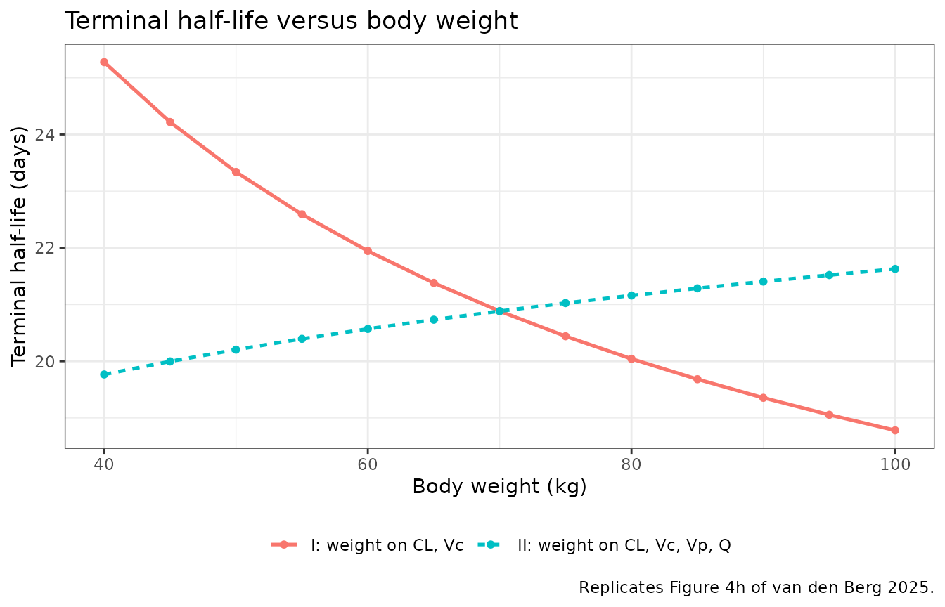
at40 <- allo_thalf |> filter(WT == 40)

tibble::tibble(
  Combination = at40$combination,
  `Simulated t1/2 at 40 kg (day)` = at40$t_half,
  `Published t1/2 at 40 kg (day)` = c(24.4, 19.0)
) |>
  mutate(`% diff` = (`Simulated t1/2 at 40 kg (day)` /
                       `Published t1/2 at 40 kg (day)` - 1) * 100) |>
  knitr::kable(
    digits = 2,
    caption = "Terminal half-life at 40 kg versus van den Berg 2025 Results 'Covariate model'."
)| Combination | Simulated t1/2 at 40 kg (day) | Published t1/2 at 40 kg (day) | % diff |
|---|---|---|---|
| I: weight on CL, Vc | 25.28 | 24.4 | 3.59 |
| II: weight on CL, Vc, Vp, Q | 19.77 | 19.0 | 4.04 |
pct_longer <- 100 * (at40$t_half[1] / at40$t_half[2] - 1)
cat(sprintf(
  "Combination I is %.1f%% longer than combination II at 40 kg (paper: 28%%)\n",
  pct_longer
))
#> Combination I is 27.9% longer than combination II at 40 kg (paper: 28%)
stopifnot(abs(pct_longer - 28) < 3)

# The crossover direction is the paper's point: at 40 kg combination I gives the
# LONGER half-life, at 100 kg the SHORTER one.
at100 <- allo_thalf |> filter(WT == 100)
stopifnot(at40$t_half[1] > at40$t_half[2], at100$t_half[1] < at100$t_half[2])
Exposure, by PKNCA
The paper adds that “after a single 100 mg dose, total drug exposure in a 40 kg individual was only 10% higher with combination 2 compared to combination I”, and that the difference is eliminated after multiple doses. The integration window behind that 10% is not stated; it is reproduced below over a three-cycle (63-day) window, which is the horizon Figure S7C-E displays.
allo_nca_input <- allo |>
  filter(!is.na(Cc)) |>
  mutate(arm = paste(combination, WT, sep = " @ ")) |>
  select(arm, id = WT, time, Cc)

allo_conc <- PKNCA::PKNCAconc(
  allo_nca_input, Cc ~ time | arm + id, concu = "mg/L", timeu = "day"
)
allo_dose <- PKNCA::PKNCAdose(
  distinct(allo_nca_input, arm, id) |> mutate(time = 0, amt = 100),
  amt ~ time | arm + id, doseu = "mg"
)

allo_res <- PKNCA::pk.nca(PKNCA::PKNCAdata(
  allo_conc, allo_dose,
  intervals = data.frame(
    start = 0, end = c(63, Inf),
    aucall = c(TRUE, FALSE), aucinf.obs = c(FALSE, TRUE),
    half.life = c(FALSE, TRUE)
  )
))

allo_summary <- as.data.frame(allo_res) |>
  filter(PPTESTCD %in% c("aucall", "aucinf.obs", "half.life")) |>
  tidyr::separate_wider_delim(arm, " @ ", names = c("combination", "wt_lab")) |>
  select(combination, WT = id, PPTESTCD, PPORRES) |>
  tidyr::pivot_wider(names_from = PPTESTCD, values_from = PPORRES)

exposure_ratio <- allo_summary |>
  filter(WT == 40) |>
  summarise(
    `AUC0-63d ratio (II / I)` =
      aucall[startsWith(combination, "II")] / aucall[startsWith(combination, "I:")],
    `AUC0-inf ratio (II / I)` =
      aucinf.obs[startsWith(combination, "II")] / aucinf.obs[startsWith(combination, "I:")]
  )

knitr::kable(
  exposure_ratio, digits = 3,
  caption = "Exposure ratio at 40 kg after a single 100 mg IV dose. The paper's ~10% figure is reproduced over the 63-day (three q3w cycle) window; extrapolated to infinity the two configurations differ by only ~3%, which is the paper's 'eliminated after multiple doses' observation, since AUC over a dosing interval at steady state equals Dose/CL and the two CL exponents differ by only 0.06."
)| AUC0-63d ratio (II / I) | AUC0-inf ratio (II / I) |
|---|---|
| 1.112 | 1.034 |
stopifnot(
  exposure_ratio$`AUC0-63d ratio (II / I)` > 1.05,
  exposure_ratio$`AUC0-63d ratio (II / I)` < 1.20
)
allo_summary |>
  filter(WT %in% c(40, 70, 100)) |>
  arrange(combination, WT) |>
  rename(
    "Combination" = combination, "Weight (kg)" = WT,
    "AUC0-63d (mg*day/L)" = aucall,
    "AUC0-inf (mg*day/L)" = aucinf.obs,
    "t1/2 (day)" = half.life
  ) |>
  knitr::kable(
    digits = 2,
    caption = "PKNCA parameters for the two weight-covariate configurations. At 70 kg the two are identical by construction, since both reduce to the across-model medians."
)| Combination | Weight (kg) | AUC0-63d (mg*day/L) | t1/2 (day) | AUC0-inf (mg*day/L) |
|---|---|---|---|---|
| I: weight on CL, Vc | 40 | 559.73 | 25.21 | 668.80 |
| I: weight on CL, Vc | 70 | 403.29 | 20.82 | 454.56 |
| I: weight on CL, Vc | 100 | 323.71 | 18.72 | 355.39 |
| II: weight on CL, Vc, Vp, Q | 40 | 622.39 | 19.71 | 691.63 |
| II: weight on CL, Vc, Vp, Q | 70 | 403.29 | 20.82 | 454.56 |
| II: weight on CL, Vc, Vp, Q | 100 | 305.67 | 21.56 | 347.87 |
At 70 kg both configurations must collapse onto the un-scaled generic disposition parameters:
Between-model versus between-subject variability
One of the paper’s central observations is that the spread of parameter estimates across published models is comparable to the between-subject variability within a model – which is what motivates using medians as a priori estimates in the first place. That between-model spread is a property of the literature, not of the generic model, so it is not encoded in the model file; it is tabulated here for reference (Results “Structural PK estimates” and “Stochastic model”, Figures 1c,d and 3).
tibble::tribble(
  ~Parameter, ~`Between-model CV% (Figure 1)`, ~`Between-subject CV%, base models (Figure 3b)`,
  "CL", 54.6, 43.0,
  "Vc", 25.0, 28.8,
  "Vp", 73.9, NA_real_,
  "Q",  108.0, NA_real_,
  "ka", 34.0, NA_real_,
  "F",  61.0, NA_real_
) |>
  knitr::kable(
    caption = "Variability in population estimates across the 160 models, next to the median between-subject variability reported in the base models. Only CL and Vc have both."
)| Parameter | Between-model CV% (Figure 1) | Between-subject CV%, base models (Figure 3b) |
|---|---|---|
| CL | 54.6 | 43.0 |
| Vc | 25.0 | 28.8 |
| Vp | 73.9 | NA |
| Q | 108.0 | NA |
| ka | 34.0 | NA |
| F | 61.0 | NA |
Assumptions and deviations
-
This is a meta-analysis, and the model it produces is a
meta-analytic construct. Every value is a median over published
model estimates, not an estimate from data. All parameters are
consequently
fixed(), matching the paper’s own NONMEM control stream, in which every$THETAand$OMEGAline carriesFIX. Do not read theini()values as fitted point estimates. -
The random effects are between-SUBJECT, not
between-study. This is a meta-analysis of models
rather than a regression meta-analysis of trial summaries, and the
authors deliberately used the median published between-subject omegas as
individual-level IIV in a 500-individual simulation. They therefore
carry the standard
etal<param>names rather than theeta_study_*MBMA convention. The separate between-model spread (table above) is not encoded. - Cohort size. The paper used 500 virtual individuals; this vignette uses 200 per arm, the validation-vignette cap. The residual disagreement in the half-life percentiles (a few percent) is Monte-Carlo noise from the smaller, differently-seeded sample.
-
Intravenous dosing is a bolus here. The paper notes
that in the collected models “i.v. doses are administered directly into
the central compartment over the course of an hour”, but its own
generic-model control stream (Suppl. M5) carries no infusion rate, so a
bolus is used. Over a 21-day half-life the choice is immaterial except
at the first few observations, and it makes
Cmax = Dose/Vcan exact identity to test against. -
kaunits. The abstract prints the absorption rate constant as “0.25 L/d”, which is dimensionally impossible. The Figure 5c caption and the Supplementary M5$THETAcomment both give/d, and that is what the model uses. -
Residual error is a placeholder, not an estimate.
The paper introduced no RUV. The generic model carries the control
stream’s
propSd = 1e-5verbatim; the two allometric configurations, which the paper ran “without inter-individual variability or residual variability”, carry a structuralpropSd = 0. Re-specify a residual-error model before fitting data with any of the three. -
Specimen is unstated. The 160 source models pool
serum and plasma assays (the paper reports only the detection method,
ELISA or electrochemiluminescence).
compartmentDatarecordsserumwithverified = FALSEbecause the source does not state a matrix for the generic model. - The third common covariate configuration is not extracted. The paper identifies “weight and sex on CL and Vc” (19 models) as the third most common combination but neither simulates it nor reports the median coefficients for that subset, so it cannot be parameterised from the available sources.
-
Screened but unused covariates. Median effects for
body weight, albumin, sex and ADA status across the 160 models are
recorded in the generic model’s
covariatesDataExcludedmetadata (allometric exponents 0.62 on CL and 0.56 on Vc when estimated; albumin power -0.90 on CL at a 40 g/L reference; 19% higher CL in males; 1.39-fold CL in ADA-positive patients). None of them is part of the generic model, and the paper does not report a joint covariate model that combines them, so none is encoded inmodel(). - Nonlinear and time-dependent elimination are out of scope by construction. 47.5% of the collected models included nonlinear kinetics and 19.4% time-dependent clearance, and the paper shows the linear CL component is 26% lower in mixed models (0.18 versus 0.25 L/day). The generic model describes linear IgG homeostasis only; a target-mediated component must be added explicitly for any mAb where it matters.
- The 10% single-dose exposure claim depends on an unstated integration window. It reproduces over a 63-day window (Figure S7’s display horizon) but not to infinity, where the difference is ~3%. Both numbers are shown above rather than picking the flattering one.