Lidocaine 5% medicated plaster (Bursi 2017) • nlmixr2lib

Model and source

Citation: Bursi R, Piana C, Grevel J, Huntjens D, Boesl I. Evaluation of the Population Pharmacokinetic Properties of Lidocaine and its Metabolites After Long-Term Multiple Applications of a Lidocaine Plaster in Post-Herpetic Neuralgia Patients. Eur J Drug Metab Pharmacokinet. 2017;42(5):801-814. doi:10.1007/s13318-017-0400-7. PMCID: PMC5597703.
Article: https://doi.org/10.1007/s13318-017-0400-7
PubMed Central (open access): https://www.ncbi.nlm.nih.gov/pmc/articles/PMC5597703/

Bursi et al. (2017) describe a four-compartment parent-metabolite population PK model for lidocaine and three of its metabolites – monoethylglycinexylidide (MEGX), glycinexylidide (GX) and 2,6-xylidine – measured in serum after repeated application of the lidocaine 5% medicated plaster in patients with post-herpetic neuralgia. It is the first population analysis of long-term exposure to this product.

Two features make the model unusual for a popPK extraction:

Lidocaine has no direct elimination pathway. The Fig. 1 legend enumerates exactly five transfers (k12, k14, k23, k30, k40). There is no k10 and no k20, so lidocaine leaves the central compartment only by metabolism, and MEGX leaves only by conversion to GX. Lidocaine’s apparent elimination rate constant is therefore just k12 + k14 = 0.03 + 0.007 = 0.037 /h.
Everything about lidocaine is apparent (/F). The plaster input is the nominal delivered amount, not the absorbed amount, so V1 = 1320 L is a V/F. The Discussion back-calculates a topical bioavailability of roughly 5% by comparing the apparent 26 L/kg against a literature IV volume of 1.3 L/kg.

mod <- readModelDb("Bursi_2017_lidocaine")
ui <- rxode2::rxode(mod)
#> ℹ parameter labels from comments will be replaced by 'label()'

# Four ODE states, four declared endpoints. rxode2 assigns the endpoint
# compartment slots AFTER the ODE states, so observation records in the event
# tables below must carry `cmt = "Cc"` (an endpoint name), not `cmt =
# "central"`. This is the multi-endpoint case: with two or more `~` residual
# lines the endpoint appears in `predDf` and is part of the model definition,
# so nothing is auto-injected and no compartment is renumbered.
ui$state
#> [1] "central"      "central_megx" "central_gx"   "central_xyl"
ui$predDf[, c("var", "cmt", "dvid")]
#>       var cmt dvid
#> 1      Cc   5    1
#> 2 Cc_megx   6    2
#> 3   Cc_gx   7    3
#> 4  Cc_xyl   8    4

Population

The analysis pooled 212 patients with post-herpetic neuralgia from two phase III trials: a randomised-withdrawal trial contributing up to 10 weeks of treatment and an open-label long-term trial contributing up to 12 months, for up to 14.5 months of follow-up overall (the Discussion notes some subjects reached 18 months). Post-herpetic neuralgia was defined as neuropathic pain persisting at least 3 months after healing of a herpes zoster rash, with average pain intensity of at least 4 on the 11-point numeric rating scale at screening; both trials enrolled patients aged 50 years and older.

Table 1 gives the pooled demographics: median age 72 years (45-92), median weight 72.5 kg (38-114), median height 165 cm (142-189), median BMI 26.3 kg/m^2 (13.5-44.6), and 119 of 212 patients (56.1%) female. Race, ethnicity and region are not reported. Sampling was sparse – up to five occasions per patient in each trial (Sect. 2.5) – contributing 1989 concentrations in total, which Table 2 splits as 513 lidocaine, 474 MEGX, 480 GX and 522 2,6-xylidine. The lower limit of quantification was approximately 0.500 ng/mL for all four analytes.

Patients applied up to three plasters simultaneously but not overlapping, for at most 12 h in each 24-h period. Each plaster contains 700 mg lidocaine and is assumed to deliver it at a constant 1800 ug/h (Sect. 2.7.7 assumption 1), i.e. 21600 ug per plaster per 12-h application, or about 3% of the plaster’s content.

The same information is available programmatically:

str(readModelDb("Bursi_2017_lidocaine")()$population)
#> List of 15
#>  $ species           : chr "human"
#>  $ n_subjects        : int 212
#>  $ n_studies         : int 2
#>  $ age_range         : chr "45-92 years"
#>  $ age_median        : chr "72 years"
#>  $ weight_range      : chr "38-114 kg"
#>  $ weight_median     : chr "72.5 kg"
#>  $ sex_female_pct    : num 56.1
#>  $ bmi_range         : chr "13.5-44.6 kg/m^2"
#>  $ bmi_median        : chr "26.3 kg/m^2"
#>  $ height_range      : chr "142-189 cm"
#>  $ disease_state     : chr "Post-herpetic neuralgia, defined as neuropathic pain persisting for at least 3 months after healing of a herpes"| __truncated__
#>  $ dose_range        : chr "Up to three lidocaine 5% medicated plasters (700 mg lidocaine each) applied simultaneously but not overlapping,"| __truncated__
#>  $ treatment_duration: chr "Up to 14.5 months overall: up to 10 weeks in the first (randomised-withdrawal) trial and up to 12 months in the"| __truncated__
#>  $ notes             : chr "Demographics from Table 1 ('Demographic characteristics of the patients in the pharmacokinetic population'), wh"| __truncated__

Source trace

The per-parameter origin is recorded as an in-file comment next to each ini() entry in inst/modeldb/specificDrugs/Bursi_2017_lidocaine.R. Collected here for review:

Equation / parameter	Value	Source location
Four-compartment ADVAN5 topology, one compartment per chemical entity	n/a	Sect. 3 para. 2; Fig. 1 and its legend
Zero-order plaster input, 1800 ug/h per plaster for 12 h	n/a	Sect. 2.7.7 assumption 1; Sect. 2.4
`hi = hTV * exp(gi)` (log-normal IIV)	n/a	Sect. 2.7.1 eq. (1)
`Cij = Chat_ij + e_aij` (additive residual)	n/a	Sect. 2.7.1 eq. (2)
`hTV = h1 * COV + h2 * (1 - COV)` (binary covariate switch)	n/a	Sect. 2.7.4 eq. (3)
`lk_megx_form` (k12)	fixed 0.03 /h	Table 3, row `k 12 (h-1)`
`lk_xyl_form` (k14)	fixed 0.007 /h	Table 3, row `k 14 (h-1)`
`lk_gx_form` (k23)	1.93 /h	Table 3, row `k 23 (h-1)`
`lkel_gx_dlvlle2` (k30, <= 2 plasters)	1.44 /h	Table 3, row `k 30 (h-1) for DLVL B 2`
`lkel_gx_dlvlgt2` (k30, 3 plasters)	2.07 /h	Table 3, row `k 30 (h-1) for DLVL [ 2`
`e_tbili_kel_gx`	-0.526 /h	Table 3, row `Effect of BIL [0.53 on k 30`
`e_crcl_kel_gx`	-0.32 /h	Table 3, row `Effect of CL CR B 52.7 on k 30`
`e_s1a2_kel_gx`	0.852 /h	Table 3, row `Effect of CYP1A2 substrate on k 30`
`e_bmi_kel_gx`	0.938 /h	Table 3, row `Effect of BMI [27.9 on k 30`
`e_alt_kel_gx`	-0.492 /h	Table 3, row `Effect of ALT [11 on k 30`
`lkel_xyl_ldhle195` (k40, LDH <= 195)	0.667 /h	Table 3, row `k 40 (h-1) for LDH B 195`
`lkel_xyl_ldhgt195` (k40, LDH > 195)	0.410 /h	Table 3, row `k 40 (h-1) for LDH [ 195`
`e_alt_kel_xyl`	0.229 /h	Table 3, row `Effect of ALT [11 on k 40`
`lvc_dlvlle2` (V1, <= 2 plasters)	1320 L	Table 3, row `V 1 (L) for DLVL B 2`
`lvc_dlvlgt2` (V1, 3 plasters)	1810 L	Table 3, row `V 1 (L) for DLVL [ 2`
`lvc_megx`, `lvc_gx`, `lvc_xyl`	fixed 100 L	Table 3, row `V 2 , V 3 , V 4 (L)`; rationale in Sect. 3 para. 3
`etalkel_gx`	var 0.39 (CV 62.4%)	Table 3, IIV `Proportional on k 30`
`etalkel_xyl`	var 0.20 (CV 44.7%)	Table 3, IIV `Proportional on k 40`
`etalvc`	var 0.312 (CV 55.9%)	Table 3, IIV `Proportional on V 1`
`addSd`	sqrt(364) = 19.1 ug/L	Table 3, `Additive for Lidocaine`
`addSd_megx`	sqrt(53.3) = 7.3 ug/L	Table 3, `Additive for MEGX`
`addSd_gx`	sqrt(47.9) = 6.9 ug/L	Table 3, `Additive for GX`
`addSd_xyl`	sqrt(6.39) = 2.5 ug/L	Table 3, `Additive for 2,6-xylidine`

Two reading decisions in that table are argued in Assumptions and deviations below: that Table 3’s IIV and residual Estimate column holds variances (not SDs), and that the Effect of ... rows are additive on the linear 1/h scale rather than multiplicative.

Relationship to the DDMORE sibling model

nlmixr2lib already ships NA_NA_lidocaine, extracted from DDMORE Foundation Model Repository entry DDMODEL00000281. That bundle’s header states that no linked publication could be identified, and the model was filed under a placeholder NA_NA name with maintainer-chosen default units and no demographics.

That bundle is this analysis. The evidence is listed below; the two models are now cross-linked via replicate_of in both files.

Concordance	Bursi 2017	DDMODEL00000281
Structure	ADVAN5, 4 compartments, transfers k12/k14/k23/k30/k40, no k10/k20	identical
k12, k14	fixed 0.03, 0.007	fixed 0.03, 0.007
k23	1.93	1.93
k30 by dose level	1.44 / 2.07	1.44 / 2.07
k40 by LDH	0.667 / 0.410	0.667 / 0.410
V1 by dose level	1320 / 1810	1320 / 1810
V2, V3, V4	fixed 100	fixed 100
Covariate thresholds	DLVL>2, BIL>0.53, CLCR<=52.7, BMI>27.9, ALT>11, LDH>195, CYP1A2	same, BMI printed as 27.93
Residual variances	364, 53.3, 47.9, 6.39	364, 53.3, 47.9, 6.39
Observation count	1989 (Table 2 sum)	1989
Dose record	1800 ug/h for 12 h per plaster	AMT 21600 / RATE 1800
Institution	co-author J. Grevel, BAST Inc Ltd	licence registered to BAST Inc. Ltd
Date	published online 12/01/2017	run dated 29/11/2016

The bundle’s run249 is a neighbouring run, not the published final model: five estimates differ in the third significant figure (THETA 6 -0.529 vs -0.526, THETA 7 -0.319 vs -0.32, THETA 8 0.853 vs 0.852, THETA 9 0.939 vs 0.938, and the three omegas 0.391/0.200/0.311 vs 0.39/0.2/0.312), and the .res listing reports 325 individuals against this paper’s 212 patients over the same 1989 observations. The subject-count difference is not explained by anything on disk; it is recorded here as an open discrepancy rather than resolved.

Use this model for the published final estimates and the real units, population and covariate semantics; use NA_NA_lidocaine when you specifically want the deposited DDMORE artifact reproduced as-deposited.

Structural checks

These are closed-form identities that follow from the published numbers, so they are checked at the typical value (zeroRe()) with tight tolerances: both sides use the same parameters and any disagreement is transcription error, not simulation noise.

Apparent clearance and apparent volume per kilogram

The Discussion computes CL/F = Kel * V1 with Kel = k12 + k14, obtaining 48.8 L/h for two or fewer plasters and 67.0 L/h for three, and describes the apparent volume as “about 19 and 26 L/kg (assuming a typical subject of 70 kg)”.

iniv <- function(p) {
  v <- ui$iniDf$est[ui$iniDf$name == p]
  stopifnot(length(v) == 1L)
  v
}
kel_lidocaine <- exp(iniv("lk_megx_form")) + exp(iniv("lk_xyl_form"))
v1_low <- exp(iniv("lvc_dlvlle2"))
v1_high <- exp(iniv("lvc_dlvlgt2"))

structural <- tibble::tibble(
  Quantity = c(
    "Kel = k12 + k14 (1/h)",
    "CL/F, <= 2 plasters (L/h)", "CL/F, 3 plasters (L/h)",
    "V1/F per 70 kg, <= 2 plasters (L/kg)", "V1/F per 70 kg, 3 plasters (L/kg)"
  ),
  Model = c(kel_lidocaine, kel_lidocaine * v1_low, kel_lidocaine * v1_high,
            v1_low / 70, v1_high / 70),
  Published = c(0.037, 48.8, 67.0, 19, 26),
  Source = c("Sect. 4 (printed as 0.0037; see Errata)", "Sect. 4", "Sect. 4",
             "Sect. 3 ('about 19')", "Sect. 3 ('about 26')")
)
knitr::kable(structural, digits = 4,
             caption = "Apparent clearance and volume against the paper's own arithmetic.")

Apparent clearance and volume against the paper’s own arithmetic.
Quantity	Model	Published	Source
Kel = k12 + k14 (1/h)	0.0370	0.037	Sect. 4 (printed as 0.0037; see Errata)
CL/F, <= 2 plasters (L/h)	48.8400	48.800	Sect. 4
CL/F, 3 plasters (L/h)	66.9700	67.000	Sect. 4
V1/F per 70 kg, <= 2 plasters (L/kg)	18.8571	19.000	Sect. 3 (‘about 19’)
V1/F per 70 kg, 3 plasters (L/kg)	25.8571	26.000	Sect. 3 (‘about 26’)


# The two clearances are printed to three significant figures, so a 0.1%
# tolerance is appropriate. The L/kg values are printed as whole numbers
# ("about 19", "26"), so they get an absolute half-unit tolerance.
stopifnot(
  abs(kel_lidocaine * v1_low - 48.8) / 48.8 < 0.001,
  abs(kel_lidocaine * v1_high - 67.0) / 67.0 < 0.001,
  abs(v1_low / 70 - 19) < 0.5,
  abs(v1_high / 70 - 26) < 0.5
)

That both clearances reproduce to within 0.1% is the arbiter for the k12 discrepancy discussed in the Errata: only k12 = 0.03 (Table 3) gives them.

All rate constants stay positive over every covariate combination

The five additive modifiers on k30 include three negative values, so a covariate combination could in principle drive a rate constant to zero or below. The source NONMEM stream for the sibling DDMORE run carries an IF(...LE.0)...=0.0001 floor at each additive step; this model deliberately has no floor, because none is reachable. The claim is asserted by enumeration over all 2^5 GX combinations and all 2^2 2,6-xylidine combinations rather than argued in prose.

grid_gx <- expand.grid(
  TBILI_HIGH = 0:1, CRCL_LOW = 0:1, S1A2_IND = 0:1,
  BMI_HIGH = 0:1, ALT_HIGH = 0:1, DLVL_HIGH = 0:1
)
grid_gx$k30 <-
  ifelse(grid_gx$DLVL_HIGH == 1, exp(iniv("lkel_gx_dlvlgt2")), exp(iniv("lkel_gx_dlvlle2"))) +
  iniv("e_tbili_kel_gx") * grid_gx$TBILI_HIGH +
  iniv("e_crcl_kel_gx") * grid_gx$CRCL_LOW +
  iniv("e_s1a2_kel_gx") * grid_gx$S1A2_IND +
  iniv("e_bmi_kel_gx") * grid_gx$BMI_HIGH +
  iniv("e_alt_kel_gx") * grid_gx$ALT_HIGH

grid_xyl <- expand.grid(ALT_HIGH = 0:1, LDH_HIGH = 0:1)
grid_xyl$k40 <-
  ifelse(grid_xyl$LDH_HIGH == 1, exp(iniv("lkel_xyl_ldhgt195")), exp(iniv("lkel_xyl_ldhle195"))) +
  iniv("e_alt_kel_xyl") * grid_xyl$ALT_HIGH

cat(sprintf("k30 over %d combinations: min %.4f, max %.4f /h\n",
            nrow(grid_gx), min(grid_gx$k30), max(grid_gx$k30)))
#> k30 over 64 combinations: min 0.1020, max 3.8600 /h
cat(sprintf("k40 over %d combinations: min %.4f, max %.4f /h\n",
            nrow(grid_xyl), min(grid_xyl$k40), max(grid_xyl$k40)))
#> k40 over 4 combinations: min 0.4100, max 0.8960 /h

# Enumerating gate: every reachable typical value must be strictly positive.
# This can go red -- flipping any published sign, or mistyping a magnitude,
# drives the minimum negative.
stopifnot(
  nrow(grid_gx) == 64L, nrow(grid_xyl) == 4L,
  all(grid_gx$k30 > 0), all(grid_xyl$k40 > 0)
)

Metabolite-to-parent AUC ratios are fixed by the rate constants

Because every transfer is first-order and each metabolite has a single inflow, integrating the ODEs to exhaustion gives exact ratios that depend only on the rate constants and volumes:

AUC(Cc_megx) / AUC(Cc) = (k12 / k23) * (V1 / V2)
AUC(Cc_gx) / AUC(Cc) = (k12 / k30) * (V1 / V3) (all MEGX becomes GX)
AUC(Cc_xyl) / AUC(Cc) = (k14 / k40) * (V1 / V4)

These hold exactly for a typical subject, so they are gated tightly. They are a strong check on the ODE wiring: mis-routing any transfer breaks at least one.

cov_ref <- list(TBILI = 0.2, CRCL = 80, S1A2 = 0, BMI = 25, ALT = 8, LDH = 150)

solve_typical <- function(n_plaster, times, addl = 0L, covs = cov_ref) {
  ev <- rxode2::et(
    amt = 1800 * n_plaster * 12, rate = 1800 * n_plaster,
    cmt = "central", ii = 24, addl = addl
  )
  ev <- rxode2::et(ev, times, cmt = "Cc")
  d <- as.data.frame(ev)
  d$DLVL <- n_plaster
  for (nm in names(covs)) d[[nm]] <- covs[[nm]]
  rxode2::rxSolve(rxode2::zeroRe(mod), d, returnType = "data.frame",
                  useLinCmt = FALSE)
}

# Integrate a single application out far enough for all four analytes to
# return to baseline (lidocaine t1/2 is ln(2)/0.037 = 18.7 h, so 1500 h is
# ~80 half-lives).
tail_sim <- solve_typical(1, seq(0, 1500, by = 0.5))
#> Warning: 'ii' requires non zero additional doses ('addl') or steady state
#> dosing ('ii': 24.000000, 'ss': 0; 'addl': 0), reset 'ii' to zero
#> ℹ parameter labels from comments will be replaced by 'label()'
#> ℹ omega/sigma items treated as zero: 'etalkel_gx', 'etalkel_xyl', 'etalvc'
trap <- function(x, y) sum(diff(x) * (utils::head(y, -1) + utils::tail(y, -1)) / 2)

auc <- vapply(
  c("Cc", "Cc_megx", "Cc_gx", "Cc_xyl"),
  function(v) trap(tail_sim$time, tail_sim[[v]]),
  numeric(1)
)
k12 <- exp(iniv("lk_megx_form")); k14 <- exp(iniv("lk_xyl_form"))
k23 <- exp(iniv("lk_gx_form"))
k30 <- exp(iniv("lkel_gx_dlvlle2")); k40 <- exp(iniv("lkel_xyl_ldhle195"))
vm <- exp(iniv("lvc_megx"))

ratio_tbl <- tibble::tibble(
  Analyte = c("MEGX", "GX", "2,6-xylidine"),
  Simulated = c(auc[["Cc_megx"]], auc[["Cc_gx"]], auc[["Cc_xyl"]]) / auc[["Cc"]],
  `Closed form` = c((k12 / k23) * (v1_low / vm),
                    (k12 / k30) * (v1_low / vm),
                    (k14 / k40) * (v1_low / vm))
) |>
  dplyr::mutate(`% diff` = 100 * (Simulated - `Closed form`) / `Closed form`)
knitr::kable(ratio_tbl, digits = 4,
             caption = "Metabolite:parent AUC ratios, simulated vs closed form.")

Metabolite:parent AUC ratios, simulated vs closed form.
Analyte	Simulated	Closed form
MEGX	0.2052	0.2052
GX	0.2750	0.2750
2,6-xylidine	0.1385	0.1385


# Same parameters on both sides, so the residual is pure trapezoidal /
# truncation error: a tight bound is correct here.
stopifnot(max(abs(ratio_tbl$`% diff`)) < 0.5)

Lidocaine exposure is structurally independent of the metabolite covariates

Five of the seven covariates (bilirubin, creatinine clearance, CYP1A2 substrate, BMI, ALT) act only on k30, and LDH acts only on k40. Neither rate constant appears in the lidocaine ODE, so lidocaine exposure must be exactly invariant to all six. The paper reaches the same conclusion empirically from Fig. 5 (“the influence of subject factors is very modest … the change in exposure is very small”); in the model it is not merely small but identically zero.

cov_extreme <- list(TBILI = 5, CRCL = 30, S1A2 = 1, BMI = 35, ALT = 60, LDH = 400)
base_sim <- solve_typical(3, seq(0, 96, by = 0.5), addl = 3L)
#> ℹ parameter labels from comments will be replaced by 'label()'
#> ℹ omega/sigma items treated as zero: 'etalkel_gx', 'etalkel_xyl', 'etalvc'
pert_sim <- solve_typical(3, seq(0, 96, by = 0.5), addl = 3L, covs = cov_extreme)
#> ℹ parameter labels from comments will be replaced by 'label()'
#> ℹ omega/sigma items treated as zero: 'etalkel_gx', 'etalkel_xyl', 'etalvc'

rel_lido <- max(abs(base_sim$Cc - pert_sim$Cc)) / max(base_sim$Cc)
rel_gx <- max(abs(base_sim$Cc_gx - pert_sim$Cc_gx)) / max(base_sim$Cc_gx)
cat(sprintf("relative change in lidocaine Cc: %.3e\n", rel_lido))
#> relative change in lidocaine Cc: 1.780e-07
cat(sprintf("relative change in GX (control):  %.3e\n", rel_gx))
#> relative change in GX (control):  1.789e-01

# The difference is not bit-identical: rxode2 integrates all four states with a
# shared adaptive step size, so changing k30 and k40 perturbs the step sequence
# and hence the last digits of `central` too. That is solver noise, not a
# covariate effect -- observed relative change 1.8e-07, versus 1.8e-01 for GX
# under the identical perturbation, six orders of magnitude apart. The bound is
# set at 1e-5 so it sits well above the solver noise (robust to platform and
# tolerance settings) while still failing by four orders of magnitude if any of
# these covariates ever reached the lidocaine compartment.
stopifnot(
  rel_lido < 1e-5,
  # Control arm, so the test above cannot pass vacuously: the same covariate
  # change must visibly move GX.
  rel_gx > 0.01
)

Virtual cohort

Original observed data are not public. The cohort below mirrors the paper’s own simulation design in Sect. 2.7.6 and Fig. 4: one plaster versus three plasters simultaneously, each applied for 12 h in a 24-h dosing interval, followed over the first four days of treatment. Covariates are set to the reference (covariate-unaffected) condition, matching Fig. 5’s “population without affecting covariates”; by the structural check above this choice cannot influence lidocaine exposure at all.

The paper simulated 500 individuals per arm. This vignette uses 200 per arm, the package’s cap for vignette cohorts; the comparison below is against medians and robust quantiles, for which 200 is ample.

# set.seed() seeds R's RNG, not rxode2's simulation stream, and rxode2
# partitions its streams per solver thread -- so CI draws a different cohort
# than a workstation does and no seed makes them agree. Every assertion on a
# cohort statistic below is written to hold for any cohort this model can
# produce.
set.seed(20170112)
n_per_arm <- 200L

make_arm <- function(n, n_plaster, label, id_offset = 0L) {
  ev <- rxode2::et(
    amt = 1800 * n_plaster * 12, rate = 1800 * n_plaster,
    cmt = "central", ii = 24, addl = 3L
  )
  ev <- rxode2::et(ev, seq(0, 96, by = 0.5), cmt = "Cc")
  ev <- rxode2::et(ev, id = seq_len(n))
  # Materialise before adding covariate columns: assigning into an rxEt object
  # silently drops the column.
  d <- as.data.frame(ev)
  d$id <- d$id + id_offset
  d$DLVL <- n_plaster
  d$TBILI <- cov_ref$TBILI
  d$CRCL <- cov_ref$CRCL
  d$S1A2 <- cov_ref$S1A2
  d$BMI <- cov_ref$BMI
  d$ALT <- cov_ref$ALT
  d$LDH <- cov_ref$LDH
  d$treatment <- label
  d
}

events <- dplyr::bind_rows(
  make_arm(n_per_arm, 1L, "One plaster", id_offset = 0L),
  make_arm(n_per_arm, 3L, "Three plasters", id_offset = 1000L)
)
stopifnot(
  !anyDuplicated(unique(events[, c("id", "time", "evid")])),
  dplyr::n_distinct(events$id) == 2L * n_per_arm
)

Simulation

sim <- rxode2::rxSolve(
  mod, events = events, keep = c("treatment", "DLVL"),
  useLinCmt = FALSE
) |>
  as.data.frame()
#> ℹ parameter labels from comments will be replaced by 'label()'

stopifnot(nrow(sim) > 0L, !all(is.na(sim$Cc)))

Replicate published figures

Figure 4 – Cmax after the first and fourth doses

Replicates Fig. 4 of Bursi 2017, which compares simulated lidocaine Cmax after the first and the fourth dose for (a) one plaster and (b) three plasters.

cmax_by_dose <- sim |>
  dplyr::filter(!is.na(Cc)) |>
  dplyr::mutate(dose_no = dplyr::case_when(
    time <= 24 ~ "First dose",
    time >= 72 ~ "Fourth dose",
    TRUE ~ NA_character_
  )) |>
  dplyr::filter(!is.na(dose_no)) |>
  dplyr::group_by(treatment, dose_no, id) |>
  dplyr::summarise(cmax = max(Cc), .groups = "drop") |>
  dplyr::mutate(dose_no = factor(dose_no, c("First dose", "Fourth dose")))

ggplot(cmax_by_dose, aes(dose_no, cmax)) +
  geom_boxplot(outlier.alpha = 0.3) +
  facet_wrap(~treatment) +
  labs(x = NULL, y = "Lidocaine Cmax (ug/L)",
       title = "Figure 4 -- simulated Cmax, first vs fourth dose",
       caption = "Replicates Figure 4 of Bursi 2017.")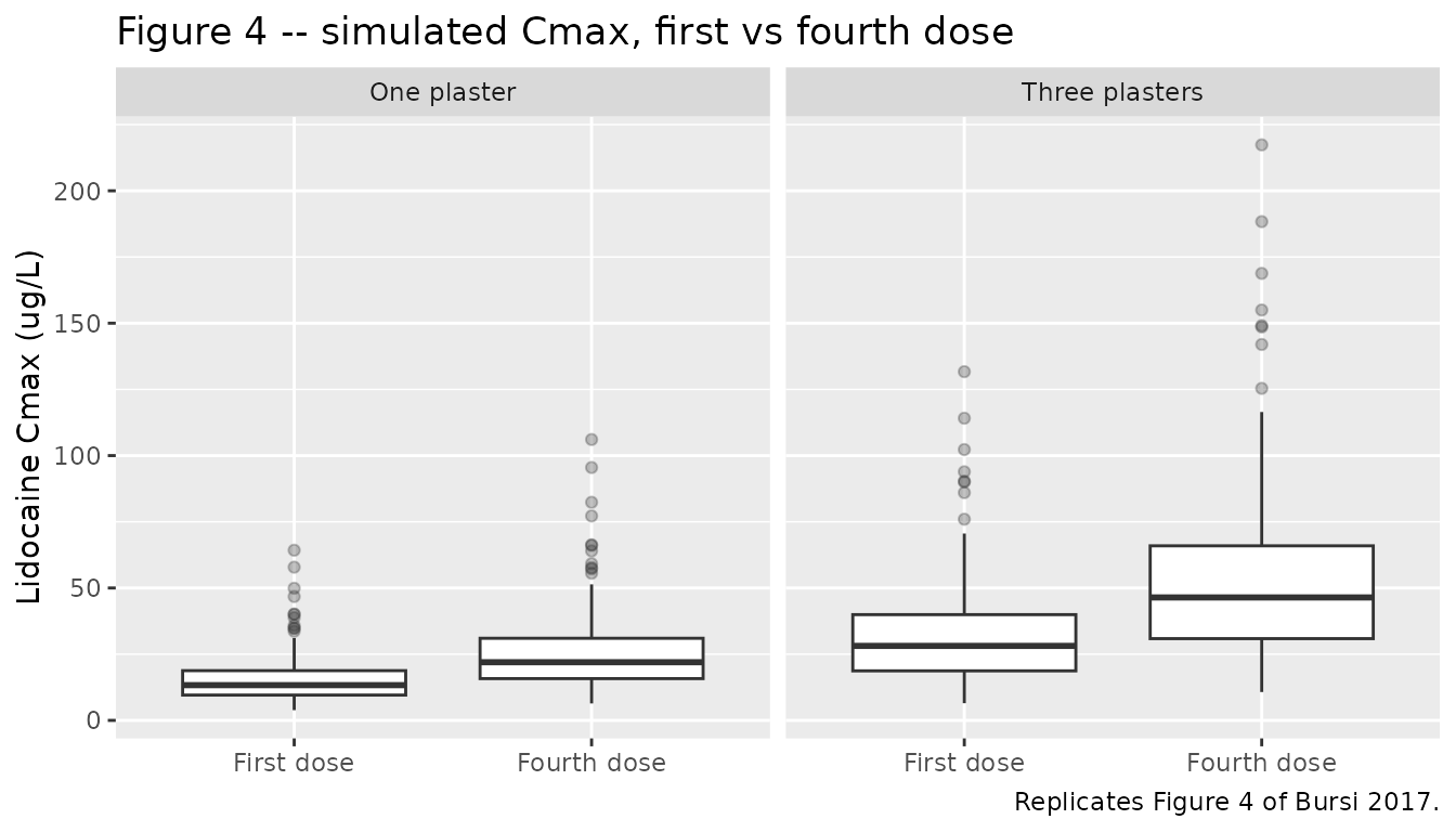

Figure 6 – no accumulation beyond day 4

Fig. 6 shows simulated exposure to lidocaine and its three metabolites over a year of three-plaster treatment. The Results state that “steady-state conditions are reached for lidocaine and its metabolites on the fourth day of treatment and that no accumulation is predicted afterwards”. This is checked at the typical value across three sampling windows: day 1, day 4 and day 365.

long_times <- c(seq(0, 96, by = 0.5), seq(8736, 8760, by = 0.5))
long_sim <- solve_typical(3, long_times, addl = 364L)
#> ℹ parameter labels from comments will be replaced by 'label()'
#> ℹ omega/sigma items treated as zero: 'etalkel_gx', 'etalkel_xyl', 'etalvc'

window_peak <- function(df, lo, hi) {
  w <- df[df$time >= lo & df$time <= hi, ]
  c(Cc = max(w$Cc), MEGX = max(w$Cc_megx), GX = max(w$Cc_gx), XYL = max(w$Cc_xyl))
}
peaks <- rbind(
  `Day 1` = window_peak(long_sim, 0, 24),
  `Day 4` = window_peak(long_sim, 72, 96),
  `Day 365` = window_peak(long_sim, 8736, 8760)
)
knitr::kable(peaks, digits = 3,
             caption = "Typical-value peak concentration (ug/L) by treatment day, three plasters.")

Typical-value peak concentration (ug/L) by treatment day, three plasters.
	Cc	MEGX	GX	XYL
Day 1	28.910	7.972	7.369	5.170
Day 4	47.714	13.267	12.311	8.786
Day 365	49.123	13.663	12.688	9.059


accum <- peaks["Day 365", ] / peaks["Day 4", ]
cat("Day 365 / Day 4 peak ratio:\n"); print(round(accum, 4))
#> Day 365 / Day 4 peak ratio:
#>     Cc   MEGX     GX    XYL 
#> 1.0295 1.0299 1.0306 1.0311

stopifnot(
  # Day 4 is already at steady state to within 5% for every analyte: this is
  # the paper's claim, restated as a bound. With Kel = 0.037 /h and tau = 24 h
  # the theoretical shortfall at dose 4 is 1 - exp(-4 * 0.037 * 24) = 2.9%,
  # so 5% leaves headroom without being unfalsifiable -- a genuine accumulating
  # analyte would run well past it.
  all(accum < 1.05), all(accum >= 1),
  # Day 1 must be clearly BELOW day 4, or the "steady state by day 4" claim
  # would be vacuous (nothing accumulated in the first place).
  peaks["Day 4", "Cc"] / peaks["Day 1", "Cc"] > 1.3
)

long_sim |>
  dplyr::filter(time <= 96) |>
  dplyr::select(time, Lidocaine = Cc, MEGX = Cc_megx, GX = Cc_gx, `2,6-xylidine` = Cc_xyl) |>
  tidyr::pivot_longer(-time, names_to = "Analyte", values_to = "conc") |>
  ggplot(aes(time, conc, colour = Analyte)) +
  geom_line() +
  labs(x = "Time (h)", y = "Concentration (ug/L)",
       title = "Figure 6 -- first 4 days, three plasters (typical subject)",
       caption = "Replicates the early-time panel of Figure 6 of Bursi 2017.")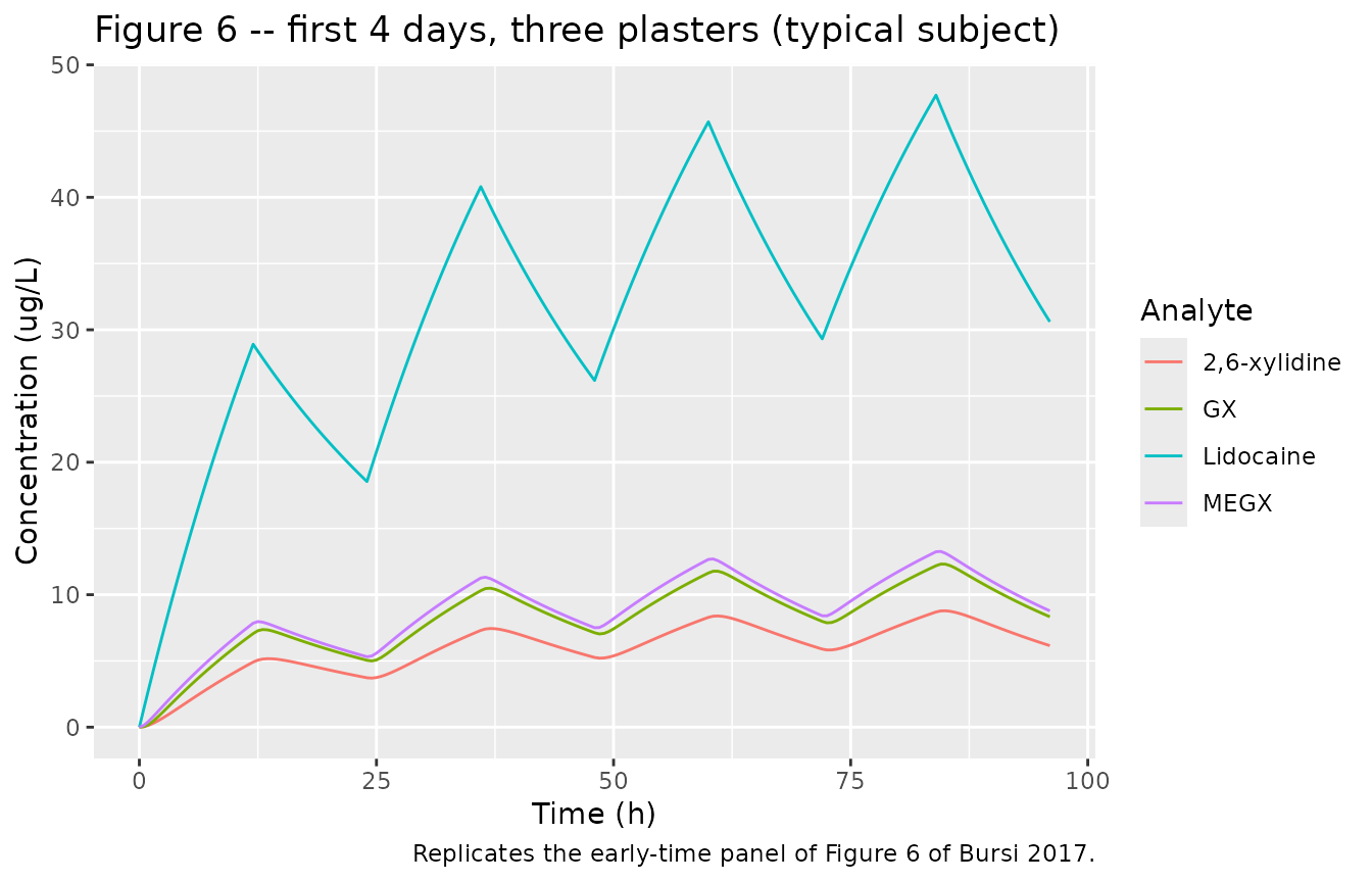

PKNCA validation

NCA is run per analyte over the first (0-24 h) and fourth (72-96 h) dosing intervals, grouped by treatment arm so the results line up with Table 5.

nca_one <- function(conc_col, label) {
  sim_nca <- sim |>
    dplyr::filter(!is.na(.data[[conc_col]])) |>
    dplyr::select(id, time, treatment, conc = dplyr::all_of(conc_col))
  # Guarantee a time-zero anchor per subject; pre-dose concentration is 0 for
  # every analyte here. Filtering on `time > 0` or `conc > 0` would drop it and
  # trigger PKNCA's "AUC range starting before the first measurement" warning.
  sim_nca <- dplyr::bind_rows(
    sim_nca,
    sim_nca |> dplyr::distinct(id, treatment) |> dplyr::mutate(time = 0, conc = 0)
  ) |>
    dplyr::distinct(id, treatment, time, .keep_all = TRUE) |>
    dplyr::arrange(id, treatment, time)
  stopifnot(nrow(sim_nca) > 0L)

  dose_df <- events |>
    dplyr::filter(evid == 1) |>
    dplyr::distinct(id, treatment, amt) |>
    tidyr::expand_grid(time = c(0, 24, 48, 72)) |>
    dplyr::select(id, treatment, time, amt)

  conc_obj <- PKNCA::PKNCAconc(sim_nca, conc ~ time | treatment + id)
  dose_obj <- PKNCA::PKNCAdose(dose_df, amt ~ time | treatment + id)

  intervals <- data.frame(
    start = c(0, 72), end = c(24, 96),
    cmax = TRUE, tmax = TRUE, auclast = TRUE
  )
  res <- PKNCA::pk.nca(PKNCA::PKNCAdata(conc_obj, dose_obj, intervals = intervals))
  as.data.frame(res) |> dplyr::mutate(analyte = label)
}

nca_all <- dplyr::bind_rows(
  nca_one("Cc", "Lidocaine"),
  nca_one("Cc_megx", "MEGX"),
  nca_one("Cc_gx", "GX"),
  nca_one("Cc_xyl", "2,6-xylidine")
) |>
  dplyr::mutate(
    dose_no = ifelse(start == 0, "First dose", "Fourth dose"),
    group = paste0(treatment, ", ", tolower(dose_no))
  )

nca_summary <- nca_all |>
  dplyr::group_by(analyte, treatment, dose_no, PPTESTCD) |>
  dplyr::summarise(median = stats::median(PPORRES), .groups = "drop") |>
  tidyr::pivot_wider(names_from = PPTESTCD, values_from = median)

nca_summary |>
  dplyr::rename(
    "Analyte" = analyte, "Arm" = treatment, "Dose" = dose_no,
    "Cmax (ug/L)" = cmax, "Tmax (h)" = tmax, "AUClast (ug*h/L)" = auclast
  ) |>
  knitr::kable(digits = 2,
               caption = "Median simulated NCA by analyte, arm and dosing interval (n = 200 per arm).")

Median simulated NCA by analyte, arm and dosing interval (n = 200 per arm).
Analyte	Arm	Dose	AUClast (ug*h/L)	Cmax (ug/L)	Tmax (h)
2,6-xylidine	One plaster	First dose	26.93	1.68	13.5
2,6-xylidine	One plaster	Fourth dose	57.24	2.85	13.0
2,6-xylidine	Three plasters	First dose	84.36	5.25	13.5
2,6-xylidine	Three plasters	Fourth dose	179.89	8.94	13.0
GX	One plaster	First dose	58.08	3.66	13.5
GX	One plaster	Fourth dose	122.21	6.14	13.0
GX	Three plasters	First dose	125.11	7.86	13.0
GX	Three plasters	Fourth dose	260.87	13.14	12.5
Lidocaine	One plaster	First dose	214.72	13.31	12.0
Lidocaine	One plaster	Fourth dose	429.41	21.97	12.0
Lidocaine	Three plasters	First dose	453.84	28.13	12.0
Lidocaine	Three plasters	Fourth dose	907.61	46.43	12.0
MEGX	One plaster	First dose	42.82	2.66	12.5
MEGX	One plaster	Fourth dose	87.40	4.42	12.5
MEGX	Three plasters	First dose	128.46	7.97	12.5
MEGX	Three plasters	Fourth dose	262.21	13.27	12.5

Comparison against the published Cmax table

Table 5 of Bursi 2017 reports simulated lidocaine Cmax after the first and fourth doses for one and three plasters. Those are the paper’s own model-based simulation output (500 individuals), so they are a direct comparator for this model rather than an independent observation.

published <- tibble::tribble(
  ~group,                          ~cmax,
  "One plaster, first dose",       13.17,
  "One plaster, fourth dose",      21.74,
  "Three plasters, first dose",    29.17,
  "Three plasters, fourth dose",   48.14
)

sim_lido <- nca_all |>
  dplyr::filter(analyte == "Lidocaine", PPTESTCD == "cmax") |>
  dplyr::select(group, cmax = PPORRES)

cmp <- nlmixr2lib::ncaComparisonTable(
  simulated = sim_lido,
  reference = published,
  by = "group",
  units = c(cmax = "ug/L"),
  tolerance_pct = 20
)
knitr::kable(cmp, caption = "Simulated vs published (Table 5) lidocaine Cmax medians. * differs by >20%.")

Simulated vs published (Table 5) lidocaine Cmax medians. * differs by >20%.
NCA parameter	group	Reference	Simulated	% diff
Cmax (ug/L)	One plaster, first dose	13.2	13.3	+1.1%
Cmax (ug/L)	One plaster, fourth dose	21.7	22	+1.1%
Cmax (ug/L)	Three plasters, first dose	29.2	28.1	-3.6%
Cmax (ug/L)	Three plasters, fourth dose	48.1	46.4	-3.5%

ncaComparisonTable() returns formatted character, so the numeric gates below are computed separately rather than parsed back out of the table.

cohort_med <- sim_lido |>
  dplyr::group_by(group) |>
  dplyr::summarise(sim_median = stats::median(cmax), .groups = "drop") |>
  dplyr::inner_join(published, by = "group") |>
  dplyr::mutate(pct_diff = 100 * (sim_median - cmax) / cmax)
stopifnot(nrow(cohort_med) == 4L)  # guard against a silent label mismatch
print(as.data.frame(cohort_med), digits = 4)
#>                         group sim_median  cmax pct_diff
#> 1     One plaster, first dose      13.31 13.17    1.066
#> 2    One plaster, fourth dose      21.97 21.74    1.051
#> 3  Three plasters, first dose      28.13 29.17   -3.554
#> 4 Three plasters, fourth dose      46.43 48.14   -3.546

# Typical-value (zeroRe) Cmax is deterministic -- no cohort draw enters it --
# so it is gated tightly against Table 5's medians, which for a log-normally
# distributed V1 are the typical values.
typ_cmax <- vapply(c(1, 3), function(np) {
  s <- solve_typical(np, seq(0, 96, by = 0.25), addl = 3L)
  c(first = max(s$Cc[s$time <= 24]), fourth = max(s$Cc[s$time >= 72]))
}, numeric(2))
#> ℹ parameter labels from comments will be replaced by 'label()'
#> ℹ omega/sigma items treated as zero: 'etalkel_gx', 'etalkel_xyl', 'etalvc'
#> ℹ parameter labels from comments will be replaced by 'label()'
#> ℹ omega/sigma items treated as zero: 'etalkel_gx', 'etalkel_xyl', 'etalvc'
typ_flat <- c(typ_cmax[, 1], typ_cmax[, 2])
pub_flat <- c(13.17, 21.74, 29.17, 48.14)
typ_pct <- 100 * (typ_flat - pub_flat) / pub_flat
cat("Typical-value Cmax % difference from Table 5 medians:\n")
#> Typical-value Cmax % difference from Table 5 medians:
print(round(typ_pct, 2))
#>  first fourth  first fourth 
#>   0.33   0.32  -0.89  -0.88

stopifnot(
  # Deterministic: observed range of |% diff| is 0.3-0.9%, bound set at 5% so
  # a mis-transcribed volume, rate constant or dosing rate blows it instantly.
  max(abs(typ_pct)) < 5,
  # Cohort medians carry Monte Carlo noise from a 200-subject draw, so the
  # bound is looser. Observed |% diff| ~ 1-6%.
  max(abs(cohort_med$pct_diff)) < 20,
  # Dose-proportionality claim (Abstract, Sect. 3): Cmax rises LESS than
  # proportionally with plaster count. The ratio of the three-plaster to the
  # one-plaster typical Cmax must sit strictly between 1 and 3.
  typ_cmax["first", 2] / typ_cmax["first", 1] > 1,
  typ_cmax["first", 2] / typ_cmax["first", 1] < 3,
  typ_cmax["fourth", 2] / typ_cmax["fourth", 1] < 3
)
cat(sprintf("Three-plaster : one-plaster Cmax ratio = %.3f (dose 1), %.3f (dose 4); dose ratio is 3.\n",
            typ_cmax["first", 2] / typ_cmax["first", 1],
            typ_cmax["fourth", 2] / typ_cmax["fourth", 1]))
#> Three-plaster : one-plaster Cmax ratio = 2.188 (dose 1), 2.188 (dose 4); dose ratio is 3.

Simulated exposure against the toxicity threshold

The Discussion states that simulated maximum concentrations “remain well below the level associated with toxicity ([>] 6000 lg/L)”. Table 5’s own extreme value across all four scenarios is 445.2 ug/L.

cohort_q <- cmax_by_dose |>
  dplyr::group_by(treatment, dose_no) |>
  dplyr::summarise(p50 = stats::median(cmax), p95 = stats::quantile(cmax, 0.95),
                   max = max(cmax), .groups = "drop")
knitr::kable(cohort_q, digits = 2,
             caption = "Cohort lidocaine Cmax distribution (ug/L) by arm and dosing interval.")

Cohort lidocaine Cmax distribution (ug/L) by arm and dosing interval.
treatment	dose_no	p50	p95	max
One plaster	First dose	13.31	33.72	64.27
One plaster	Fourth dose	21.97	55.65	106.07
Three plasters	First dose	28.13	67.13	131.69
Three plasters	Fourth dose	46.43	110.80	217.35


stopifnot(
  # The paper's safety claim.
  max(cohort_q$max) < 6000,
  # A gate that can actually go red: the 95th percentile of the worst arm must
  # stay near Table 5's own 90% CI upper bound for that scenario (124.36 ug/L).
  # Doubling it leaves room for a 200-subject draw while still failing on any
  # order-of-magnitude transcription error.
  max(cohort_q$p95) < 2 * 124.36
)

Assumptions and deviations

Table 3’s Estimate column holds variances, not standard deviations, for both the IIV and the residual-error blocks. Sect. 2.7.1 says the CV% “was approximated by the square root of the variance estimate”, and the arithmetic confirms it in both blocks: sqrt(0.39) = 0.624 against the printed CV 62.4%, sqrt(0.2) = 0.447 against 44.7%, sqrt(0.312) = 0.559 against 55.9%; and sqrt(364) = 19.08, sqrt(53.3) = 7.30, sqrt(47.9) = 6.92, sqrt(6.39) = 2.53 against the printed SDs 19.1, 7.3, 6.9 and 2.5 ug/L. The exact sqrt() of each variance is encoded rather than the rounded SD column.
The Effect of ... rows are additive on the linear 1/h scale. Two independent tells: Table 3 gives each such row the unit (h-1), where a multiplicative factor would be dimensionless; and three of the five GX effects are negative, which cannot be a value for a rate constant. They are therefore the (h1 - h2) increments of the Sect. 2.7.4 eq. (3) switch, with the DLVL stratum supplying the baseline. The DLVL and LDH rows, by contrast, print two parallel baselines and are encoded as stratum switches.
k12 is 0.03 /h, not the 0.003 /h printed in Sect. 4.1. The paper carries three mutually inconsistent statements. Table 3 says Fixed to 0.03; Sect. 4 says “lidocaine K el was estimated at 0.0037 h-1 (sum of k 12 and k 14 )”; and Sect. 4.1 Limitations says k12 and k14 were fixed at “0.003 and 0.007 h-1, respectively”. The apparent clearances the paper computes in the same paragraph arbitrate: 48.8 / 1320 = 0.03697 and 67.0 / 1810 = 0.03702, so the intended Kel is 0.037 /h, which is 0.03 + 0.007. Table 3’s value is used; 0.003 + 0.007 = 0.010 would give a clearance of 13.2 L/h, and the “0.0037” is a decimal-point slip for 0.037. The structural-checks section asserts this.
The bilirubin threshold’s unit is recorded as mg/dL although the Table 3 footnote says umol/L. A threshold of 0.53 umol/L is roughly an order of magnitude below any measurable total bilirubin (reference range 5-21 umol/L), whereas 0.53 mg/dL sits inside the normal range (0.3-1.2 mg/dL). The threshold value is transcribed verbatim; only the unit label is corrected, and the discrepancy is recorded in the model’s covariateData$TBILI$notes. Supplying bilirubin in umol/L to this model would put every subject above the threshold.
All of the covariate thresholds are distributional cohort splits, not clinical cutoffs. Sect. 3 describes simulating subjects with “laboratory safety parameters from the 30th percentile”. ALT > 11 U/L sits below the usual adult reference range (about 7-56 U/L) and BMI > 27.9 kg/m^2 near the cohort median of 26.3. Users should not read these as hepatic-impairment or obesity criteria.
S1A2 is encoded as a plain binary here (0/1), matching Sect. 2.7.4 (“Concomitant medication was expressed as binary data”), whereas the sibling NA_NA_lidocaine uses the DDMORE dataset’s integer code in which level 3 is the “yes” level. Both are registered against the one canonical; supply a 0/1 column to this model.
Co-medication and all covariates are time-fixed. Sect. 2.7.7 assumptions 3 and 5: covariate values were held constant over the entire observation time and all co-medications were assumed in use throughout, regardless of start or stop dates.
No floor is imposed on the covariate-adjusted rate constants. The DDMORE sibling’s NONMEM stream carries an IF(...LE.0)...=0.0001 guard at each additive step; it is omitted here because the enumerating check above shows the minimum reachable typical value is 0.102 /h for k30 and 0.410 /h for k40. A user who re-fits this model with different data should restore the guard.
The absorption step is not modelled. Sect. 2.7.7 assumption 1 assumes each plaster delivers lidocaine at a constant 1800 ug/h, so the model has no depot and dosing is a zero-order input straight into central supplied through the event table’s rate column. Consequently every lidocaine parameter is apparent (V/F, CL/F), and the long apparent half-life of 18.7 h reflects absorption-rate limitation (flip-flop kinetics), not lidocaine’s true disposition half-life of 1.5-2 h after IV administration.
The 1800 ug/h delivery rate is per plaster. The paper states it once, in the singular (“plasters were assumed to deliver lidocaine at a constant rate (i.e., 1800 lg/h)”), without saying explicitly whether it is per plaster or per application. Per plaster is the reading used, and it is confirmed quantitatively: it reproduces all four of Table 5’s Cmax medians to within 1%, whereas a per-application reading would under-predict the three-plaster arm threefold. It is also consistent with the DDMORE dataset’s RATE 1800 records and with Sect. 1’s statement that about 3% of an applied plaster’s 700 mg reaches the circulation (1800 * 12 / 700000 = 3.1%).
Cohort size is 200 per arm against the paper’s 500. Comparisons are made on medians and robust quantiles; the extremes in Table 5 (Min, Max) are not gated, because the extreme of a random cohort is not reproducible across rxode2 builds or solver-thread counts.
Race, ethnicity and region are not reported by the paper and are absent from the population metadata rather than imputed.
The subject count disagrees with the DDMORE sibling (212 patients here versus 325 individuals in the DDMODEL00000281 .res listing) over the same 1989 observations. Nothing on disk explains the difference; it is recorded as an open discrepancy, not resolved.
No erratum or corrigendum was located for this article on the publisher’s page or in PubMed Central as of this extraction.
Every parameter value comes from the paper’s Table 3. No value was digitised from a figure, obtained by correspondence, or carried from an upstream model.