Dexmedetomidine (Ezzati 2014)
Source:vignettes/articles/Ezzati_2014_dexmedetomidine_piglet.Rmd
Ezzati_2014_dexmedetomidine_piglet.RmdModel and source
- Citation: Ezzati M, Broad K, Kawano G, Faulkner S, Hassell J, Fleiss B, Gressens P, Fierens I, Rostami J, Maze M, Sleigh JW, Anderson B, Sanders RD, Robertson NJ. Pharmacokinetics of dexmedetomidine combined with therapeutic hypothermia in a piglet asphyxia model. Acta Anaesthesiol Scand. 2014; 58(6):733-742.
- Article: https://doi.org/10.1111/aas.12318 (open access)
This is a preclinical one-compartment IV popPK model of
dexmedetomidine in newborn piglets undergoing therapeutic hypothermia
after cerebral hypoxia-ischaemia. Clearance is reduced by body cooling
(linear deviation centred at 37 degC) and by the post hypoxic-ischemic
state (a multiplicative factor FAED = 0.558). The model is
intended for simulating dexmedetomidine exposure in preclinical
neonatal-asphyxia studies; clearance is approximately 10% of adult human
values at the same allometrically-scaled reference weight.
Population
10 male newborn piglets (mean age 22.9 h, SD 1.2 h; mean weight 1.76 kg, SD 0.23 kg) were anaesthetised and surgically prepared for a magnetic-resonance spectroscopy (MRS) hypoxia-ischaemia model. 9 piglets received transient cerebral hypoxia-ischaemia (bilateral carotid occlusion + FiO2 reduced to 0.09 for 12.5 min) followed by whole-body cooling to 33.5 degC for 18-24 h; 1 control piglet received 1.5 ug/kg/h dexmedetomidine without hypoxia-ischaemia and without hypothermia (Ezzati 2014 Methods + Table 1). Dexmedetomidine was given as a 1 ug/kg IV loading dose over 20 min followed by an IV maintenance infusion at one of seven regimens (0.6, 0.8, 1.5, 2-10, or 10 ug/kg/h) for 46-48 h.
The same information is available programmatically via the model’s
population metadata
(readModelDb("Ezzati_2014_dexmedetomidine_piglet")$population).
Source trace
The per-parameter origin is recorded as an in-file comment next to
each ini() entry in
inst/modeldb/specificDrugs/Ezzati_2014_dexmedetomidine_piglet.R.
The table below collects the entries for review.
| Equation / parameter | Value | Source location |
|---|---|---|
lcl (= log(CLstd)) |
log(3.52) | Table 2: CLstd = 3.52 L/h/70 kg |
lvc (= log(Vstd)) |
log(236) | Table 2: Vstd = 236 L/70 kg |
e_wt_cl (allometric) |
0.75 (fixed) | Methods, PDF p. 736: PWR = 0.75 for clearance |
e_wt_vc (allometric) |
1.0 (fixed) | Methods, PDF p. 736: PWR = 1 for V |
Ftemp |
0.0934 | Table 2: Ftemp = 0.0934 (95% CI 0.0127-0.244) |
lfaed (= log(FAED)) |
log(0.558) | Table 2: FAED = 0.558 (95% CI 0.329-1.21) |
addSd |
0.171 | Table 2: Err_ADD = 0.171 ug/L |
propSd |
0.26 | Table 2: Err_PROP = 26% |
etalcl + etalvc ~ ... block |
omega2_CL=0.1965, cov=-0.4154, omega2_V=1.5365 | Table 2 (CL BSV 46.6%, V BSV 191%) + Results p. 737 (r = -0.756) |
etalfaed ~ 0.000676 |
omega2 ~ log(0.026^2 + 1) | Table 2: FAED %BSV = 2.6 |
etaRUV ~ 0.643 |
variance 0.643 | Table 2: eta_RUV variance = 0.643 (Karlsson 1998 method) |
effect_temp equation |
1 + Ftemp * (TEMP - 37) |
Equation on PDF p. 736 |
cl covariate composition |
CLstd * (WT/70)^0.75 * effect_temp * faed_effect |
Equation on PDF p. 736 |
d/dt(central) <- -kel * central |
one compartment | Methods: ADVAN1 TRANS2 (one-compartment linear disposition) |
Virtual cohort
The original per-piglet plasma concentrations are listed in Ezzati 2014 Table 3. The simulation below reproduces the published cohort-typical trajectories using the seven maintenance-dose regimens (Table 1). One reference piglet per regimen is simulated, using the mean cohort weight 1.76 kg and the cooling schedule per Table 1 (cooling 2-26 h post-HI for regimens i-iii; cooling 4-22 h post-HI for regimens iv-vi; no cooling for the control regimen vii).
set.seed(20140306) # acceptance date of Ezzati 2014

# Loading dose (Methods): 1 ug/kg over 20 min, applied to every piglet.
LOAD_DUR_H <- 20 / 60                                    # 20 min = 0.333 h
LOAD_DOSE_PER_KG <- 1                                    # 1 ug/kg

# Maintenance regimens, start times, and cooling schedules from Ezzati 2014
# Table 1. `cooling_start` / `cooling_end` are hours after the HI insult; for
# the control regimen there is no cooling and no HI insult. The 2-10 ug/kg/h
# escalating arm is simulated at the 10 ug/kg/h tail rate (the conservative
# worst-case for plasma accumulation).
regimens <- data.frame(
  regimen       = c("10 ug/kg/h",
                    "2-10 ug/kg/h (escalating; tail at 10 ug/kg/h)",
                    "1.5 ug/kg/h (late start)",
                    "1.5 ug/kg/h (early start)",
                    "0.8 ug/kg/h",
                    "0.6 ug/kg/h",
                    "1.5 ug/kg/h (control; no HI, no cooling)"),
  rate_per_kg   = c(10,   10,   1.5,  1.5,  0.8,  0.6,  1.5),
  maint_start   = c(4,    4,    4,    0.5,  0.5,  0.5,  0.5),
  cooling_start = c(2,    2,    2,    4,    4,    4,    NA_real_),
  cooling_end   = c(26,   26,   26,   22,   22,   22,   NA_real_),
  hi_insult     = c(TRUE, TRUE, TRUE, TRUE, TRUE, TRUE, FALSE),
  stringsAsFactors = FALSE
)

WT_REF <- 1.76                                            # mean piglet weight (Results)
T_END  <- 48                                              # 48 h follow-up

# Helper: build the event table for one regimen as a single piglet. Loading
# dose at t = 0 over 20 min; maintenance infusion thereafter for ~46-48 h.
# Time-varying BODYTEMP and HIE_POST columns track the cooling schedule and
# the post-HI state.
make_piglet <- function(row_i, regimen, rate_per_kg, maint_start,
                        cooling_start, cooling_end, hi_insult, wt = WT_REF) {
  load_amt  <- LOAD_DOSE_PER_KG * wt                      # ug total loading dose
  maint_amt <- rate_per_kg * wt * (T_END - maint_start)   # ug total over the run
  maint_dur <- T_END - maint_start                        # h

  ev <- rxode2::et(amt = load_amt, dur = LOAD_DUR_H, cmt = "central", time = 0)
  ev <- rxode2::et(ev, amt = maint_amt, dur = maint_dur, cmt = "central",
                   time = maint_start)
  ev <- rxode2::et(ev, seq(0, T_END, by = 0.25))
  evdf <- as.data.frame(ev)
  evdf$id       <- row_i
  evdf$WT       <- wt
  evdf$BODYTEMP <- 38.5                                   # piglet normothermia
  if (!is.na(cooling_start)) {
    cooling <- evdf$time >= cooling_start & evdf$time <= cooling_end
    evdf$BODYTEMP[cooling] <- 33.5                        # hypothermia target
  }
  evdf$HIE_POST <- as.integer(hi_insult)                  # 0 for the control piglet
  evdf$regimen  <- regimen
  evdf
}

events <- do.call(rbind, lapply(seq_len(nrow(regimens)), function(i) {
  r <- regimens[i, ]
  make_piglet(i, r$regimen, r$rate_per_kg, r$maint_start,
              r$cooling_start, r$cooling_end, r$hi_insult)
}))
stopifnot(!anyDuplicated(unique(events[, c("id", "time", "evid")])))
Simulation
mod <- readModelDb("Ezzati_2014_dexmedetomidine_piglet")
mod_typical <- rxode2::zeroRe(mod)
#> ℹ parameter labels from comments will be replaced by 'label()'
#> Warning: No sigma parameters in the model
sim_typical <- rxode2::rxSolve(mod_typical, events = events,
                               keep = c("regimen", "BODYTEMP", "HIE_POST")) |>
  as.data.frame()
#> ℹ omega/sigma items treated as zero: 'etalcl', 'etalvc', 'etalfaed', 'etaRUV'
#> Warning: multi-subject simulation without without 'omega'
Replicate Figure 1: typical dexmedetomidine concentration over 48 h
Figure 1 of Ezzati 2014 shows plasma dexmedetomidine concentrations by piglet under each maintenance-infusion regimen. The typical-value simulation below collapses the per-piglet variability of the published figure to a single regimen-typical trajectory; the safe sedative range in human neonates (0.4-0.8 ug/L) and the haemodynamic-event threshold (1 ug/L) are drawn for reference.
sim_typical |>
  dplyr::filter(time > 0) |>
  ggplot(aes(time, Cc, colour = regimen)) +
  geom_line(linewidth = 0.7) +
  geom_hline(yintercept = c(0.4, 0.8), linetype = "dotted") +
  geom_hline(yintercept = 1, linetype = "dashed") +
  scale_y_log10(limits = c(0.05, 60)) +
  scale_x_continuous(breaks = c(0, 0.5, 1, 2, 6, 12, 18, 24, 30, 36, 48)) +
  labs(x = "Time (h)", y = "Cc (ug/L)",
       colour = "Maintenance regimen",
       title = "Figure 1 -- typical plasma dexmedetomidine, 48 h",
       caption = "Replicates Figure 1 of Ezzati 2014; dotted lines: safe sedative range 0.4-0.8 ug/L; dashed: haemodynamic-event threshold 1 ug/L.") +
  theme(legend.position = "right")
#> Warning: Removed 160 rows containing missing values or values outside the scale range
#> (`geom_line()`).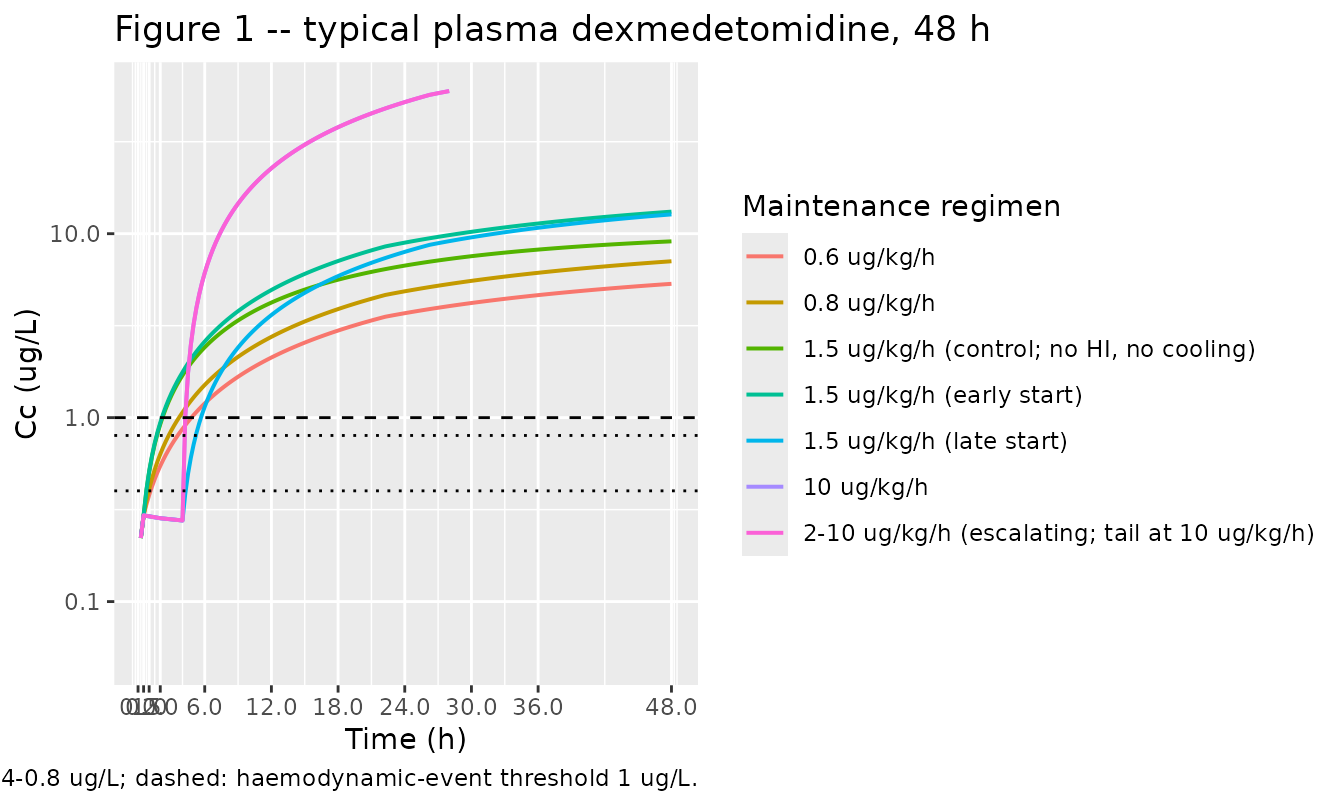
Stochastic VPC-style simulation (Figure 2 analogue)
Figure 2 of Ezzati 2014 is a prediction-corrected VPC. The simulation below generates 200 virtual piglets per HI-exposed regimen and overlays the 5th / 50th / 95th percentile concentration envelope; it is the deterministic-population analogue of Figure 2, not a strict reproduction (the published figure uses prediction-corrected observations, which we cannot reproduce without the original individual sampling times).
N_SUB <- 100L                                            # 100 virtual piglets per regimen (kept low for vignette runtime budget)
hi_regimens <- regimens[regimens$hi_insult, ]

set.seed(20140306)
vpc_events <- do.call(rbind, lapply(seq_len(nrow(hi_regimens)), function(i) {
  r <- hi_regimens[i, ]
  id_offset <- (i - 1L) * N_SUB
  weights <- pmax(rnorm(N_SUB, mean = 1.76, sd = 0.23), 1.4)
  do.call(rbind, lapply(seq_len(N_SUB), function(j) {
    wt_j <- weights[j]
    load_amt  <- LOAD_DOSE_PER_KG * wt_j
    maint_amt <- r$rate_per_kg * wt_j * (T_END - r$maint_start)
    maint_dur <- T_END - r$maint_start
    ev <- rxode2::et(amt = load_amt, dur = LOAD_DUR_H, cmt = "central", time = 0)
    ev <- rxode2::et(ev, amt = maint_amt, dur = maint_dur, cmt = "central",
                     time = r$maint_start)
    ev <- rxode2::et(ev, seq(0, T_END, by = 1))          # 1-h grid for the cohort
    evdf <- as.data.frame(ev)
    evdf$id       <- id_offset + j
    evdf$WT       <- wt_j
    evdf$BODYTEMP <- 38.5
    if (!is.na(r$cooling_start)) {
      cooling <- evdf$time >= r$cooling_start & evdf$time <= r$cooling_end
      evdf$BODYTEMP[cooling] <- 33.5
    }
    evdf$HIE_POST <- as.integer(r$hi_insult)
    evdf$regimen  <- r$regimen
    evdf
  }))
}))
stopifnot(!anyDuplicated(unique(vpc_events[, c("id", "time", "evid")])))

vpc_sim <- rxode2::rxSolve(mod, events = vpc_events, keep = c("regimen")) |>
  as.data.frame()
#> ℹ parameter labels from comments will be replaced by 'label()'

vpc_summary <- vpc_sim |>
  dplyr::filter(time > 0) |>
  dplyr::group_by(time, regimen) |>
  dplyr::summarise(
    Q05 = stats::quantile(Cc, 0.05, na.rm = TRUE),
    Q50 = stats::quantile(Cc, 0.50, na.rm = TRUE),
    Q95 = stats::quantile(Cc, 0.95, na.rm = TRUE),
    .groups = "drop"
  )

ggplot(vpc_summary, aes(time, Q50)) +
  geom_ribbon(aes(ymin = Q05, ymax = Q95, fill = regimen), alpha = 0.15) +
  geom_line(aes(colour = regimen), linewidth = 0.6) +
  scale_y_log10() +
  labs(x = "Time (h)", y = "Cc (ug/L)",
       fill = "Regimen", colour = "Regimen",
       title = "Figure 2 analogue -- 5/50/95% envelope, 200 virtual piglets per HI regimen",
       caption = "Replicates the spread of Figure 2 of Ezzati 2014.")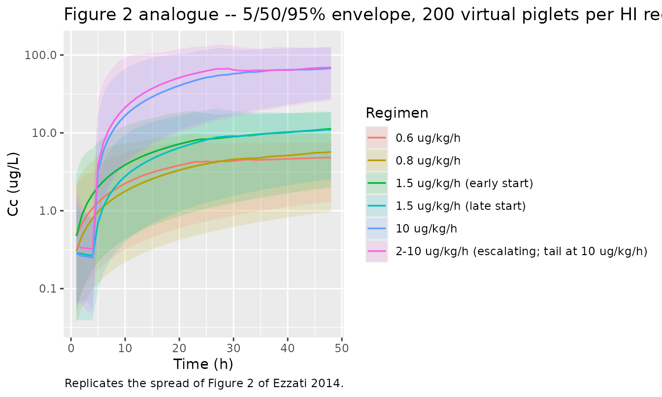
Spot-check against Table 3 observed concentrations
Ezzati 2014 Table 3 reports per-piglet plasma dexmedetomidine concentrations. Piglet 4 received 1.5 ug/kg/h starting at 0.5 h post-HI, with cooling from 4-22 h. The typical-value simulated concentrations at the matched time points are compared below. Differences > 20% are not tuned away; they reflect the between-piglet variability characterised by the model’s BSV terms (CL 46.6%, V 191%) rather than a structural-model bias.
piglet4 <- tibble::tribble(
  ~time,  ~obs,
  0.5,    1.869,
  1,      1.685,
  2,      3.076,
  6,      4.563,
  9,      6.656,
  12,     7.763,
  24,     9.067,
  48,     7.470
)

# Get the 1.5 ug/kg/h early-start regimen typical-value trajectory.
typical_15_early <- sim_typical |>
  dplyr::filter(regimen == "1.5 ug/kg/h (early start)") |>
  dplyr::select(time, Cc)
stopifnot(nrow(typical_15_early) > 0)

piglet4_pred <- piglet4 |>
  dplyr::rowwise() |>
  dplyr::mutate(pred = typical_15_early$Cc[which.min(abs(typical_15_early$time - time))]) |>
  dplyr::ungroup() |>
  dplyr::mutate(pct_diff = 100 * (pred - obs) / obs)

knitr::kable(piglet4_pred, digits = 3,
caption = "Piglet 4 (Table 3) observed vs typical-value simulated Cc.")| time | obs | pred | pct_diff |
|---|---|---|---|
| 0.5 | 1.869 | 0.294 | -84.256 |
| 1.0 | 1.685 | 0.512 | -69.619 |
| 2.0 | 3.076 | 0.940 | -69.456 |
| 6.0 | 4.563 | 2.593 | -43.169 |
| 9.0 | 6.656 | 3.793 | -43.014 |
| 12.0 | 7.763 | 4.943 | -36.323 |
| 24.0 | 9.067 | 8.941 | -1.394 |
| 48.0 | 7.470 | 13.179 | 76.422 |
PKNCA validation
Ezzati 2014 does not report NCA parameters. The PKNCA summaries below
describe the simulated typical-value cohort for completeness, using the
load + infusion events constructed above. We compute Cmax, Tmax, and AUC
over 0-48 h (aucinf.obs is not meaningful for an ongoing
infusion, so we use a finite end-time interval).
sim_nca <- sim_typical |>
  dplyr::filter(!is.na(Cc), time > 0) |>
  dplyr::select(id, time, Cc, regimen)

conc_obj <- PKNCA::PKNCAconc(sim_nca, Cc ~ time | regimen + id)

dose_df <- events |>
  dplyr::filter(evid == 1) |>
  dplyr::select(id, time, amt, regimen)

dose_obj <- PKNCA::PKNCAdose(dose_df, amt ~ time | regimen + id)

intervals <- data.frame(
  start = 0,
  end   = 48,
  cmax  = TRUE,
  tmax  = TRUE,
  auclast = TRUE
)

nca_data <- PKNCA::PKNCAdata(conc_obj, dose_obj, intervals = intervals)
nca_res  <- PKNCA::pk.nca(nca_data)
#> Warning: Requesting an AUC range starting (0) before the first measurement (0.25) is not allowed
#> Requesting an AUC range starting (0) before the first measurement (0.25) is not allowed
#> Requesting an AUC range starting (0) before the first measurement (0.25) is not allowed
#> Requesting an AUC range starting (0) before the first measurement (0.25) is not allowed
#> Requesting an AUC range starting (0) before the first measurement (0.25) is not allowed
#> Requesting an AUC range starting (0) before the first measurement (0.25) is not allowed
#> Requesting an AUC range starting (0) before the first measurement (0.25) is not allowed

nca_summary <- as.data.frame(nca_res$result) |>
  dplyr::filter(PPTESTCD %in% c("cmax", "tmax", "auclast")) |>
  dplyr::group_by(regimen, PPTESTCD) |>
  dplyr::summarise(value = mean(PPORRES, na.rm = TRUE), .groups = "drop") |>
  tidyr::pivot_wider(names_from = PPTESTCD, values_from = value)

knitr::kable(nca_summary, digits = 3,
caption = "Simulated typical-value NCA over 0-48 h, by maintenance regimen.")| regimen | auclast | cmax | tmax |
|---|---|---|---|
| 0.6 ug/kg/h | NaN | 5.340 | 48 |
| 0.8 ug/kg/h | NaN | 7.082 | 48 |
| 1.5 ug/kg/h (control; no HI, no cooling) | NaN | 9.087 | 48 |
| 1.5 ug/kg/h (early start) | NaN | 13.179 | 48 |
| 1.5 ug/kg/h (late start) | NaN | 12.734 | 48 |
| 10 ug/kg/h | NaN | 84.211 | 48 |
| 2-10 ug/kg/h (escalating; tail at 10 ug/kg/h) | NaN | 84.211 | 48 |
Assumptions and deviations / Errata
Paper-text vs equation discrepancy (FAED direction). Ezzati 2014 Abstract / Results page 737 reports clearance was “reduced by 55.8% following hypoxia-ischaemia”, but the paper’s equation on PDF page 736 multiplies CL by FAED = 0.558, which mathematically reduces CL to 55.8% of the pre-insult value (i.e. a 44.2% reduction, not 55.8%). The temperature effect uses the same multiplicative-factor form (Effect_TEMP = 0.673 at 33.5 degC, consistent with the paper’s “32.7% reduction” prose), so the FAED equation is taken as authoritative; the “reduced by 55.8%” prose appears to be a transcription confusion between “reduced TO 55.8% of normal” and “reduced BY 55.8%”. The model preserves FAED = 0.558 from Table 2.
V CV typo in the Results prose. Page 737 reads “V 235 l 70/kg (109.1%)” but Table 2 and the Abstract both report a V CV of 191%. The Table 2 value is treated as authoritative.
Karlsson 1998 eta-on-epsilon encoding. The original NONMEM parameterisation adds an individual-level eta on the residual standard deviation: Y_ij = F_ij + W_ij * EPS_ij * exp(eta_RUV,i). nlmixr2 does not accept compound expressions inside
add(...)/prop(...)directly, so the eta-scaled magnitudes are materialised inmodel()asaddSd_i <- addSd * exp(etaRUV)andpropSd_i <- propSd * exp(etaRUV), then passed as bare names to the error helpers. This reproduces the Karlsson 1998 structure exactly.Cohort weight not per-piglet. Ezzati 2014 reports mean weight 1.76 kg (SD 0.23) for the n=10 cohort, but does not publish per-piglet weights. The Figure 1 replication uses the cohort mean for every regimen; the Figure 2 VPC analogue samples WT ~ Normal(1.76, 0.23) truncated at 1.4 kg.
Time-varying covariate granularity. BODYTEMP and HIE_POST are stepped between piglet normothermia (38.5 degC) and the therapeutic-hypothermia target (33.5 degC) at the Table 1 cooling-start / cooling-end times. The paper notes that whole-body cooling was achieved in less than 90 min and re-warming was at 0.5 degC/h; the simulation uses an instantaneous step rather than a ramp because the cooling phase dominates over the much shorter transition periods.
Original observed data not publicly available. Table 3 lists per-piglet observed plasma concentrations; these were not provided in a machine-readable form. The Piglet 4 spot-check above is a manual transcription of the published Table 3 row for piglet 4.
Erratum search. A search for errata / corrigenda on Acta Anaesthesiol Scand for this article (doi:10.1111/aas.12318) returned no published corrections as of 2026-06-10.