Avalglucosidase alfa (Tuffal 2023)
Source:vignettes/articles/Tuffal_2023_avalglucosidase_alfa.Rmd
Tuffal_2023_avalglucosidase_alfa.Rmd
library(nlmixr2lib)
library(PKNCA)
#>
#> Attaching package: 'PKNCA'
#> The following object is masked from 'package:stats':
#>
#>     filter
library(rxode2)
#> rxode2 5.1.8 using 2 threads (see ?getRxThreads)
#>   no cache: create with `rxCreateCache()`
library(dplyr)
#>
#> Attaching package: 'dplyr'
#> The following objects are masked from 'package:stats':
#>
#>     filter, lag
#> The following objects are masked from 'package:base':
#>
#>     intersect, setdiff, setequal, union
library(tidyr)
library(ggplot2)
Model and source
- Citation: Tuffal G, Tiraboschi G, Hurbin F, Boittet P, Palmer R, Martinez J-M, Fabre D. Population Pharmacokinetic Modeling and Determination of Individual Exposure to Avalglucosidase Alfa in Adolescent and Adult Patients With Late-Onset Pompe Disease: Analysis of Pooled Data From Phase I to III Clinical Trials. Ther Drug Monit. 2023;45(5):644-652. doi:10.1097/FTD.0000000000001086.
- Article: https://doi.org/10.1097/FTD.0000000000001086
- Supplemental Digital Content 1 (study designs, model-development runs, typical-value exposures): http://links.lww.com/TDM/A648
Avalglucosidase alfa is an enzyme replacement therapy for Pompe disease, a lysosomal storage disorder caused by deficiency of acid alpha-glucosidase (GAA). Tuffal et al. pooled 2042 plasma drug-activity determinations from 75 patients with late-onset Pompe disease (LOPD) across three trials and fit a population PK model in NONMEM 7.4.1.
The striking feature of the data is that each dosing interval contains two chronological kinetic sequences. The first drives essentially all of the exposure: concentrations fall from the end-of-infusion peak with one slope down to roughly 10 ug/mL, then decline steeply to near the limit of quantitation between 10 and 16 hours. The second sequence is a slow, nearly flat rebound that peaks after about 72 hours at very low concentrations and stays above the LLOQ out to the next dose at 336 hours in two-thirds of patients. It contributes only about 1% of total AUC.
Model structure
The authors reproduce that shape with a concatenated (series) three-compartment model, rather than the usual parallel/mammillary layout:
            linear CL  <--+
                          |
   Michaelis-Menten   <---+
     (Vmax / Km)          |
                          |
                     [ central, V1 ] <===== Qpc (one way) ===== [ peripheral2, V3 ]
                          ^                                              ^
                          |                                              |
                          +======== Q2 (both ways) ====== [ peripheral1, V2 ]
                                                                |
                                                                +== Q3 (one way) ==>
Three properties are load-bearing:
-
Elimination is from the central compartment only,
and it is the sum of a linear clearance
CLand a parallel saturable Michaelis-Menten clearance (Vmax,Km). BecauseVmax / Km= 21.8 L/h greatly exceedsCL= 0.869 L/h, the Michaelis-Menten arm is saturated (and therefore nearly irrelevant) at the high concentrations right after the infusion, and dominant at the very low concentrations of the late phase. That asymmetry produces the steep second slope of the first kinetic sequence. -
The peripheral compartments are in series.
peripheral1exchanges bidirectionally withcentralviaQ2, butperipheral2is fed fromperipheral1(viaQ3), not fromcentral. -
Q3andQpcare one-way.Qpcreturns drug fromperipheral2straight back tocentral, closing the loop into a cycle. The slow trickle back throughQpc(0.0206 L/h, the smallest parameter in the model) is what generates the second kinetic sequence.
The one-way reading is the authors’ own, not an inference from the figure alone. Supplemental Digital Content 1 Table 2 tabulates the model-development runs, and it contains a row labelled “Q3 one way” and a row labelled “Q3 two ways”; the bidirectional variant is rejected with the verbatim comment “Markedly increased OFV”, and every subsequent development step – including the row “Final model (No allometry)” – descends from the one-way branch.
Q2, V2, Q3, and
V3 were fixed after preliminary screening and sensitivity
analysis “to avoid identifiability issues in the model” (Results). They
are wrapped in fixed() in the model file.
mod <- readModelDb("Tuffal_2023_avalglucosidase_alfa")
mod
#> function() {
#>   description <- paste(
#>     "Concatenated 3-compartment population PK model for avalglucosidase",
#>     "alfa (enzyme replacement therapy) in adolescent and adult patients",
#>     "with late-onset Pompe disease (Tuffal 2023). Pooled analysis of 2042",
#>     "plasma drug-activity determinations from 75 patients across three",
#>     "trials (phase I/II NCT01898364, its follow-up NCT02032524, and phase",
#>     "III NCT02782741) at 5, 10, and 20 mg/kg IV Q2W. Elimination from the",
#>     "central compartment is the sum of a linear clearance (CL) and a",
#>     "parallel saturable Michaelis-Menten clearance (Vmax, Km). The two",
#>     "peripheral compartments are arranged in SERIES rather than in",
#>     "parallel: central exchanges bidirectionally with peripheral1 (Q2),",
#>     "peripheral1 feeds peripheral2 one way (Q3), and peripheral2 returns",
#>     "drug directly to central one way (Qpc). That cycle is what produces",
#>     "the two chronological kinetic sequences seen in the data - a first",
#>     "exposure-driving sequence contributing about 99% of AUC, then a slow",
#>     "low-concentration rebound peaking near 87 h and remaining above the",
#>     "LLOQ out to the next dose at 336 h. The authors explicitly tested and",
#>     "rejected a bidirectional Q3 ('Markedly increased OFV'). Q2, V2, Q3,",
#>     "and V3 were fixed after preliminary screening to avoid identifiability",
#>     "problems. No covariates are retained: 12 demographic / laboratory",
#>     "covariates and 3 antidrug-antibody parameterisations were screened and",
#>     "none qualified, so the screened set is documented in",
#>     "covariatesDataExcluded rather than covariateData. Allometric scaling",
#>     "was tested and not retained, so the model carries no body-weight term."
#>   )
#>   reference <- paste(
#>     "Tuffal G, Tiraboschi G, Hurbin F, Boittet P, Palmer R,",
#>     "Martinez J-M, Fabre D. Population Pharmacokinetic Modeling and",
#>     "Determination of Individual Exposure to Avalglucosidase Alfa in",
#>     "Adolescent and Adult Patients With Late-Onset Pompe Disease:",
#>     "Analysis of Pooled Data From Phase I to III Clinical Trials.",
#>     "Ther Drug Monit. 2023;45(5):644-652.",
#>     "doi:10.1097/FTD.0000000000001086."
#>   )
#>   vignette <- "Tuffal_2023_avalglucosidase_alfa"
#>
#>   units <- list(
#>     time = "h",
#>     dosing = "mg",
#>     concentration = "ug/mL"
#>   )
#>
#>   # No covariates are retained in the final model. Every covariate the paper
#>   # screened is documented in covariatesDataExcluded below.
#>   # Issue #482: what each ODE state holds, in what amount units, in what
#>   # biological matrix. Derived mechanically; verified = FALSE means it has
#>   # NOT been checked against the source paper.
#>   compartmentData <- list(
#>     central = list(analyte = "avalglucosidase alfa", units = "mg", specimen = "plasma", verified = FALSE),
#>     peripheral1 = list(analyte = "avalglucosidase alfa", units = "mg", specimen = "plasma", verified = FALSE),
#>     peripheral2 = list(analyte = "avalglucosidase alfa", units = "mg", specimen = "plasma", verified = FALSE)
#>   )
#>
#>   covariateData <- list()
#>
#>   covariatesDataExcluded <- list(
#>     WT = list(
#>       description = "Baseline body weight. Screened as a continuous covariate on CL and V1, and separately as the scaling variable for allometric scaling of central clearance and volume (Methods, 'Population Pharmacokinetic Modeling' item 1).",
#>       units = "kg",
#>       type = "continuous",
#>       reference_category = NULL,
#>       notes = "Survived backward deletion on CL IIV (removal raised OFV by more than the 10.84 criterion) but was NOT retained: the resulting model failed the covariance-step acceptance criteria (correlated parameters and/or several RSE much greater than 50%), the effect on CL IIV was not significant, and the single-covariate bootstrap qualification failed (Results, 'Population Pharmacokinetic Model'). Allometric scaling was likewise tested and not retained, so the final model contains no body-weight term at all. Reported exposure nevertheless tracks weight: median AUC0-336h was 32% lower below 50 kg and 41% higher at or above 100 kg relative to 50-100 kg (Results, 'Patient Exposure'; Supplemental Digital Content 6). Population mean weight 75.9 kg (SD 20.1), Table 1."
#>     ),
#>     AGE = list(
#>       description = "Baseline age. Screened as a continuous demographic covariate (Methods).",
#>       units = "years",
#>       type = "continuous",
#>       reference_category = NULL,
#>       notes = "Not retained. Population mean 46.0 years (SD 15.1), Table 1; a single patient was under 18 years."
#>     ),
#>     SEXF = list(
#>       description = "Sex indicator. Screened as a categorical demographic covariate (Methods).",
#>       units = "(binary)",
#>       type = "binary",
#>       reference_category = "0 (male)",
#>       notes = "Not retained. Paper reports counts rather than an indicator column: 36 of 75 female (48%), Table 1."
#>     ),
#>     RACE_WHITE = list(
#>       description = "White / Caucasian race indicator. Part of the 'ethnicity' categorical covariate screened in the Methods.",
#>       units = "(binary)",
#>       type = "binary",
#>       reference_category = "0 (non-Caucasian)",
#>       notes = "Not retained. Table 1 reports Caucasian 68 of 75 (90.7%). The paper screened ethnicity as a single categorical covariate; it is decomposed here into the canonical one-hot indicators so the screened groups are individually documented. Table 3 labels the same variable 'Phenotype'."
#>     ),
#>     RACE_BLACK = list(
#>       description = "Black race indicator. Part of the 'ethnicity' categorical covariate screened in the Methods.",
#>       units = "(binary)",
#>       type = "binary",
#>       reference_category = "0 (not Black)",
#>       notes = "Not retained. Table 1 reports Black 2 of 75 (2.67%)."
#>     ),
#>     RACE_ASIAN = list(
#>       description = "Asian race indicator. Part of the 'ethnicity' categorical covariate screened in the Methods.",
#>       units = "(binary)",
#>       type = "binary",
#>       reference_category = "0 (not Asian)",
#>       notes = "Not retained. Table 1 reports Asian 3 of 75 (4.00%); a further 2 patients (2.67%) were recorded as 'Other'."
#>     ),
#>     CRCL = list(
#>       description = "Baseline renal function. The paper screened renal function under two parameterisations: creatinine clearance, and glomerular filtration rate estimated by the Modification of Diet in Renal Disease (MDRD) formula (Methods).",
#>       units = "mL/min/1.73 m^2",
#>       type = "continuous",
#>       reference_category = NULL,
#>       notes = "Neither parameterisation was retained. Both map to the single canonical renal-function column, which covers creatinine-based estimates and measured GFR alike; the two parameterisations are recorded here rather than split across two columns because neither entered the final model. Table 3 stratifies exposure by GFR: 64 of 70 patients at or above 90 mL/min, 6 in the 60-89 range."
#>     ),
#>     CPK = list(
#>       description = "Baseline creatine kinase. Screened as a continuous laboratory covariate (Methods).",
#>       units = "U/L",
#>       type = "continuous",
#>       reference_category = NULL,
#>       notes = "Not retained. Baseline value used, per the Methods convention 'Unless otherwise stated, the baseline value was used as the covariate.' Paper calls this 'creatine kinase'; units are not stated."
#>     ),
#>     ALP = list(
#>       description = "Baseline alkaline phosphatase. Screened as a continuous laboratory covariate (Methods).",
#>       units = "U/L",
#>       type = "continuous",
#>       reference_category = NULL,
#>       notes = "Not retained. Units not stated in the paper."
#>     ),
#>     ALT = list(
#>       description = "Baseline alanine aminotransferase. Screened as a continuous laboratory covariate (Methods).",
#>       units = "U/L",
#>       type = "continuous",
#>       reference_category = NULL,
#>       notes = "Not retained. Units not stated in the paper."
#>     ),
#>     AST = list(
#>       description = "Baseline aspartate aminotransferase. Screened as a continuous laboratory covariate (Methods).",
#>       units = "U/L",
#>       type = "continuous",
#>       reference_category = NULL,
#>       notes = "Not retained, despite surviving backward deletion on CL IIV alongside body weight (removal raised OFV by more than the 10.84 criterion). Rejected for the same reasons as WT: covariance-step acceptance criteria not met, effect on CL IIV not significant, and single-covariate bootstrap qualification failed (Results, 'Population Pharmacokinetic Model'). Units not stated in the paper."
#>     ),
#>     TBILI = list(
#>       description = "Baseline total bilirubin. Screened as a continuous laboratory covariate (Methods).",
#>       units = "umol/L",
#>       type = "continuous",
#>       reference_category = NULL,
#>       notes = "Not retained. The paper says only 'bilirubin' and states no units; total bilirubin is assumed."
#>     ),
#>     ALB = list(
#>       description = "Baseline albumin. Screened as a continuous laboratory covariate (Methods).",
#>       units = "g/L",
#>       type = "continuous",
#>       reference_category = NULL,
#>       notes = "Not retained. Units not stated in the Methods, but Table 3 stratifies exposure at a 45 g/L cut point (28 patients below, 42 at or above), which implies g/L."
#>     ),
#>     ADA_POS = list(
#>       description = "Antidrug-antibody positivity. The paper screened two of its three ADA parameterisations through this concept: a subject-level categorical covariate (ADA occurring at least once versus never during follow-up) and a longitudinal categorical covariate (positive or not at the current time).",
#>       units = "(binary)",
#>       type = "binary",
#>       reference_category = "0 (ADA-negative)",
#>       notes = "Neither parameterisation was retained. Both are recorded against this single canonical column: the ever-positive reading is time-fixed and the longitudinal reading is time-varying, but the column encoding is identical and neither entered the final model. See Methods, 'Population Pharmacokinetic Modeling', and Supplemental Digital Content 2 for the ADA assays."
#>     ),
#>     ADA_TITER = list(
#>       description = "Continuous antidrug-antibody titer. The third of the paper's three ADA parameterisations (Methods).",
#>       units = "titer (reciprocal dilution; assay described in Supplemental Digital Content 2)",
#>       type = "continuous",
#>       reference_category = NULL,
#>       notes = "Not retained. Qualitative and semiquantitative titer assays were performed for the phase III study only; two further assays characterised the neutralising ability of ADA (enzymatic-activity inhibition and uptake inhibition). Table 3 does not stratify exposure by ADA status."
#>     )
#>   )
#>
#>   population <- list(
#>     species = "human",
#>     n_subjects = 75L,
#>     n_studies = 3L,
#>     age_range = "at least 3 years by protocol eligibility; the analysis population was adolescent and adult, with 1 patient under 18 years, 59 aged 18-64, and 10 aged 65 or older among the 70 who received 20 mg/kg (Table 3)",
#>     age_median = "mean 46.0 years (SD 15.1) overall; 46.0 (16.6) in phase I/II and 46.1 (14.5) in phase III (Table 1)",
#>     weight_range = "not reported as a range; exposure was stratified below 50 kg (5 patients), 50-99 kg (55), and at or above 100 kg (10) among the 70 who received 20 mg/kg (Table 3)",
#>     weight_median = "mean 75.9 kg (SD 20.1) overall; 72.0 (14.5) in phase I/II and 77.8 (22.1) in phase III (Table 1)",
#>     sex_female_pct = 48,
#>     race_ethnicity = c(Caucasian = 90.7, Black = 2.67, Asian = 4.00, Other = 2.67),
#>     disease_state = "late-onset Pompe disease (LOPD), confirmed by GAA enzyme deficiency from any tissue source, 2 confirmed pathogenic GAA variants, or both; 14 of 75 (18.7%) had been pretreated with alglucosidase alfa for at least 9 months and 61 (81.3%) were treatment-naive",
#>     dose_range = "5, 10, or 20 mg/kg IV Q2W. Each infusion was given stepwise to limit hypersensitivity reactions: 1 mg/kg/h for 30 min, 3 mg/kg/h for 30 min, 5 mg/kg/h for 30 min, then 7 mg/kg/h until the planned dose was delivered. 70 of the 75 patients received 20 mg/kg (51 from phase III plus 19 from phase I/II who started at or shifted to the top dose).",
#>     regions = "not reported; multicentre across NCT01898364, NCT02032524, and NCT02782741",
#>     notes = "Baseline demographics are in Table 1; the per-study design, dosing, and sampling schedules are in Supplemental Digital Content 1 Table 1. Data attrition: 2374 concentrations collected, 2066 above the LLOQ, 9 removed before modelling (3 predoses above LLOQ, 1 aberrant trough, 5 from a patient with truncated prior-dose information) giving 2057, then 15 conditional-weighted-residual outliers (0.7%) removed, giving the final 2042 used for fitting. Concentrations are plasma enzymatic activity, assayed fluorometrically over a validated range of 0.0125 (LLOQ) to 3.0 ug/mL. Fit in NONMEM 7.4.1 with FOCE-I. Final-model performance: mean bias -2.66% and RMSE 30.7% for IPRED, -0.433% and 38.9% for PRED; AAFE 1.36 (IPRED) and 1.72 (PRED). Bootstrap convergence 86% of 1000 runs."
#>   )
#>
#>   ini({
#>     # Structural parameters -- Tuffal 2023 Table 2, "Fixed effects" block.
#>     # Estimated parameters (RSE reported):
#>     lcl   <- log(0.869);  label("Linear clearance from the central compartment CL (L/h)")            # Table 2: CL = 0.869 L/h (RSE 0.09%, 95% CI 0.868-0.871; bootstrap median 0.884)
#>     lvc   <- log(3.35);   label("Central compartment volume V1 (L)")                                 # Table 2: V1 = 3.35 L (RSE 0.07%, 95% CI 3.35-3.36; bootstrap median 3.44)
#>     lvmax <- log(9.82);   label("Michaelis-Menten maximum elimination rate Vmax (mg/h)")             # Table 2: Vmax = 9.82 mg/h (RSE 0.19%, 95% CI 9.79-9.86; bootstrap median 10.6)
#>     lkm   <- log(0.451);  label("Michaelis-Menten half-saturation constant Km (ug/mL)")              # Table 2: Km = 0.451 ug/mL (RSE 0.12%, 95% CI 0.450-0.452; bootstrap median 0.493)
#>     lqpc  <- log(0.0206); label("Back-redistribution clearance peripheral2 -> central Qpc (L/h)")    # Table 2: Qpc = 0.0206 L/h (RSE 0.330%, 95% CI 0.0204-0.0207; bootstrap median 0.0183)
#>
#>     # Fixed parameters. Results, "Population Pharmacokinetic Model": "To avoid
#>     # identifiability issues in the model, Q2, Q3, V2, and V3 values were fixed
#>     # after the preliminary model screening and sensitivity analysis." Table 2
#>     # marks each of these four rows "Fixed value" with no RSE, CI, or bootstrap.
#>     lq    <- fixed(log(0.254)); label("Inter-compartmental clearance central <-> peripheral1 Q2 (L/h)")  # Table 2: Q2 = 0.254 L/h (Fixed value)
#>     lvp   <- fixed(log(296));   label("First peripheral compartment volume V2 (L)")                      # Table 2: V2 = 296 L (Fixed value)
#>     lq2   <- fixed(log(1.87));  label("One-way inter-compartmental clearance peripheral1 -> peripheral2 Q3 (L/h)")  # Table 2: Q3 = 1.87 L/h (Fixed value)
#>     lvp2  <- fixed(log(1.31));  label("Second peripheral compartment volume V3 (L)")                     # Table 2: V3 = 1.31 L (Fixed value)
#>
#>     # IIV -- Tuffal 2023 Table 2, "Inter-individual variability" block. The
#>     # Estimate column carries the log-scale variance omega^2 and the
#>     # parenthesised value is the corresponding CV%. Confirmed against the
#>     # paper's own printed CV% for all five etas via CV = sqrt(exp(omega^2) - 1):
#>     #   0.0870 -> 30.2%   0.0160 -> 12.7%   0.125 -> 36.6%
#>     #   0.171  -> 43.1%   1.87   -> 234%
#>     # matching Table 2 exactly, and matching the Results sentence "IIV in model
#>     # parameters ranged from 12.7% to 43.1% for CL, V1, Vmax, and Km and up to
#>     # 234% for Qpc". Results also states "A diagonal matrix was used to explain
#>     # IIV", so there are no off-diagonal terms. "The log-normal IIV of the
#>     # parameters was used."
#>     etalcl   ~ 0.0870   # Table 2: omega^2 CL   = 0.0870 (CV 30.2%), RSE 20.5%
#>     etalvc   ~ 0.0160   # Table 2: omega^2 V1   = 0.0160 (CV 12.7%), RSE 32.1%
#>     etalvmax ~ 0.125    # Table 2: omega^2 Vmax = 0.125  (CV 36.6%), RSE 34.8%
#>     etalkm   ~ 0.171    # Table 2: omega^2 Km   = 0.171  (CV 43.1%), RSE 10.1%
#>     etalqpc  ~ 1.87     # Table 2: omega^2 Qpc  = 1.87   (CV 234%),  RSE 1.21%
#>
#>     # Residual error. Results: "the residual variability was best described
#>     # using a proportional error model". Table 2 reports sigma^2 = 0.125
#>     # (CV 35.3%); for a proportional model the SD is sqrt(0.125) = 0.3536,
#>     # which reproduces the printed 35.3% exactly. Corroborated by the
#>     # reported RMSE of 30.7% (IPRED) and 38.9% (PRED), which bracket it.
#>     propSd <- 0.354; label("Proportional residual error (fraction)")  # Table 2: residual variability sigma^2 = 0.125 (CV 35.3%), RSE 0.01% -> propSd = sqrt(0.125)
#>   })
#>
#>   model({
#>     # Individual parameters. Estimated parameters carry log-normal IIV; the
#>     # four parameters Table 2 marks "Fixed value" carry none.
#>     cl   <- exp(lcl + etalcl)
#>     vc   <- exp(lvc + etalvc)
#>     vmax <- exp(lvmax + etalvmax)
#>     km   <- exp(lkm + etalkm)
#>     qpc  <- exp(lqpc + etalqpc)
#>     q    <- exp(lq)
#>     vp   <- exp(lvp)
#>     q2   <- exp(lq2)
#>     vp2  <- exp(lvp2)
#>
#>     # Concentrations driving the clearance terms. Amounts are in mg and volumes
#>     # in L, so every concentration is in mg/L = ug/mL -- the units of Km
#>     # (0.451 ug/mL) and of the reported observations.
#>     Cc  <- central / vc
#>     Cp1 <- peripheral1 / vp
#>     Cp2 <- peripheral2 / vp2
#>
#>     # Concatenated ("series") 3-compartment system with back-redistribution,
#>     # per Tuffal 2023 Figure 1 inset and the Results parameter list "CL, Vmax,
#>     # and Km, describing the 2 parallel clearances from the central
#>     # compartment, and Q2, Q3, Qpc, V1, V2, and V3, describing drug
#>     # distribution."
#>     #
#>     #   central <--Q2--> peripheral1 --Q3--> peripheral2 --Qpc--> central
#>     #      |  linear CL (out)
#>     #      |  Michaelis-Menten Vmax/Km (out)
#>     #
#>     # Only Q2 is bidirectional. Q3 and Qpc are one-way, which is what closes
#>     # the loop and generates the second kinetic sequence. The one-way reading is
#>     # the authors' own: Supplemental Digital Content 1 Table 2 compares a
#>     # "Q3 one way" run against a "Q3 two ways" run and rejects the latter with
#>     # the comment "Markedly increased OFV"; every later development step,
#>     # including "Final model (No allometry)", descends from the one-way branch.
#>     # Elimination is from the central compartment only, and both clearances act
#>     # in parallel there.
#>     d/dt(central) <- -cl * Cc -
#>                       vmax * Cc / (km + Cc) -
#>                       q * Cc + q * Cp1 +
#>                       qpc * Cp2
#>     d/dt(peripheral1) <- q * Cc - q * Cp1 - q2 * Cp1
#>     d/dt(peripheral2) <- q2 * Cp1 - qpc * Cp2
#>
#>     Cc ~ prop(propSd)
#>   })
#> }
#> <environment: 0x55679dd0fed0>
Population
The analysis population is 75 patients with late-onset Pompe disease pooled from a phase I/II safety and tolerability study (NCT01898364, 24 patients, 5/10/20 mg/kg Q2W for 25 weeks), its open-label extension (NCT02032524, 19 of those patients, with the 5 and 10 mg/kg arms progressively shifted up to 20 mg/kg), and a phase III efficacy trial (NCT02782741, 51 treatment-naive patients at 20 mg/kg Q2W for 49 weeks). Counting the phase III patients together with the phase I/II patients who started at or shifted to the top dose, 70 of the 75 received 20 mg/kg.
Baseline characteristics (Table 1): mean age 46.0 years (SD 15.1), mean body weight 75.9 kg (SD 20.1), 36 of 75 female (48%), 90.7% Caucasian / 2.67% Black / 4.00% Asian / 2.67% Other. Fourteen patients (18.7%) had been pretreated with alglucosidase alfa for at least 9 months; 61 (81.3%) were treatment-naive.
Concentrations are plasma enzymatic activity, measured by a fluorometric assay validated from 0.0125 (LLOQ) to 3.0 ug/mL. Of 2374 concentrations collected, 2066 were above the LLOQ; 9 were removed before modelling and 15 conditional-weighted- residual outliers (0.7%) afterwards, leaving the 2042 used for the fit.
The same information is available programmatically:
str(readModelDb("Tuffal_2023_avalglucosidase_alfa")()$population)
#> List of 13
#>  $ species       : chr "human"
#>  $ n_subjects    : int 75
#>  $ n_studies     : int 3
#>  $ age_range     : chr "at least 3 years by protocol eligibility; the analysis population was adolescent and adult, with 1 patient unde"| __truncated__
#>  $ age_median    : chr "mean 46.0 years (SD 15.1) overall; 46.0 (16.6) in phase I/II and 46.1 (14.5) in phase III (Table 1)"
#>  $ weight_range  : chr "not reported as a range; exposure was stratified below 50 kg (5 patients), 50-99 kg (55), and at or above 100 k"| __truncated__
#>  $ weight_median : chr "mean 75.9 kg (SD 20.1) overall; 72.0 (14.5) in phase I/II and 77.8 (22.1) in phase III (Table 1)"
#>  $ sex_female_pct: num 48
#>  $ race_ethnicity: Named num [1:4] 90.7 2.67 4 2.67
#>   ..- attr(*, "names")= chr [1:4] "Caucasian" "Black" "Asian" "Other"
#>  $ disease_state : chr "late-onset Pompe disease (LOPD), confirmed by GAA enzyme deficiency from any tissue source, 2 confirmed pathoge"| __truncated__
#>  $ dose_range    : chr "5, 10, or 20 mg/kg IV Q2W. Each infusion was given stepwise to limit hypersensitivity reactions: 1 mg/kg/h for "| __truncated__
#>  $ regions       : chr "not reported; multicentre across NCT01898364, NCT02032524, and NCT02782741"
#>  $ notes         : chr "Baseline demographics are in Table 1; the per-study design, dosing, and sampling schedules are in Supplemental "| __truncated__
Source trace
Every ini() entry in
inst/modeldb/specificDrugs/Tuffal_2023_avalglucosidase_alfa.R
carries an in-file comment naming its source location. They are
collected here for review. All structural and variability values come
from Table 2 of the main paper.
| Equation / parameter | Value | Source location |
|---|---|---|
lcl (CL) |
0.869 L/h | Table 2, CL row (RSE 0.09%, 95% CI 0.868-0.871) |
lvc (V1) |
3.35 L | Table 2, V1 row (RSE 0.07%, 95% CI 3.35-3.36) |
lvmax (Vmax) |
9.82 mg/h | Table 2, Vmax row (RSE 0.19%, 95% CI 9.79-9.86) |
lkm (Km) |
0.451 ug/mL | Table 2, Km row (RSE 0.12%, 95% CI 0.450-0.452) |
lqpc (Qpc) |
0.0206 L/h | Table 2, Qpc row (RSE 0.330%, 95% CI 0.0204-0.0207) |
lq (Q2), fixed()
|
0.254 L/h | Table 2, Q2 row (“Fixed value”) |
lvp (V2), fixed()
|
296 L | Table 2, V2 row (“Fixed value”) |
lq2 (Q3), fixed()
|
1.87 L/h | Table 2, Q3 row (“Fixed value”) |
lvp2 (V3), fixed()
|
1.31 L | Table 2, V3 row (“Fixed value”) |
etalcl |
omega^2 = 0.0870 | Table 2, IIV block (CV 30.2%, RSE 20.5%) |
etalvc |
omega^2 = 0.0160 | Table 2, IIV block (CV 12.7%, RSE 32.1%) |
etalvmax |
omega^2 = 0.125 | Table 2, IIV block (CV 36.6%, RSE 34.8%) |
etalkm |
omega^2 = 0.171 | Table 2, IIV block (CV 43.1%, RSE 10.1%) |
etalqpc |
omega^2 = 1.87 | Table 2, IIV block (CV 234%, RSE 1.21%) |
propSd |
0.354 | Table 2, residual row: sigma^2 = 0.125 (CV 35.3%); sqrt(0.125) = 0.354 |
| Diagonal omega (no off-diagonals) | n/a | Results: “A diagonal matrix was used to explain IIV” |
| Proportional residual error | n/a | Results: “the residual variability was best described using a proportional error model” |
| Parallel linear + Michaelis-Menten elimination from central | n/a | Figure 1 inset; Results parameter list (“CL, Vmax, and Km, describing the 2 parallel clearances from the central compartment”) |
Series peripheral chain; Q3 and Qpc
one-way |
n/a | Figure 1 inset; SDC1 Table 2, “Q3 one way” vs “Q3 two ways” (“Markedly increased OFV”) |
| Four parameters fixed | n/a | Results: “Q2, Q3, V2, and V3 values were fixed after the preliminary model screening and sensitivity analysis” |
| No covariates retained | n/a | Results and Conclusions: “None of the covariates tested could explain the interindividual variability” |
| Stepwise infusion protocol | 1/3/5 mg/kg/h for 30 min each, then 7 mg/kg/h | Methods, “Study Design”; SDC1 Table 1 |
Reading the IIV column
Table 2’s IIV block reports the log-scale variance
omega^2, with the corresponding CV% in parentheses. That
reading is confirmed by the paper’s own printed CV% for all five etas
via CV = sqrt(exp(omega^2) - 1):
omega_sq <- c(CL = 0.0870, V1 = 0.0160, Vmax = 0.125, Km = 0.171, Qpc = 1.87)
published_cv_pct <- c(CL = 30.2, V1 = 12.7, Vmax = 36.6, Km = 43.1, Qpc = 234)

data.frame(
  `omega^2` = omega_sq,
  `CV% from omega^2` = round(100 * sqrt(exp(omega_sq) - 1), 1),
  `CV% published` = published_cv_pct,
  check.names = FALSE
)
#>      omega^2 CV% from omega^2 CV% published
#> CL     0.087             30.1          30.2
#> V1     0.016             12.7          12.7
#> Vmax   0.125             36.5          36.6
#> Km     0.171             43.2          43.1
#> Qpc    1.870            234.3         234.0

# Reproduces every printed CV% to the published precision, so the column is a
# log-scale variance (not an SD, and not a CV on the natural scale).
stopifnot(
  max(abs(100 * sqrt(exp(omega_sq) - 1) - published_cv_pct)) < 0.6
)
The residual row is read differently and deliberately so: for a
proportional error model sqrt(0.125) = 0.3536, which
reproduces the printed 35.3% exactly, whereas
sqrt(exp(0.125) - 1) = 0.365 would print as 36.5%. The
reported RMSE values (30.7% for IPRED, 38.9% for PRED) bracket 35.4% and
corroborate the reading.
Dosing: the stepwise infusion
Every infusion was escalated stepwise to limit infusion-associated
hypersensitivity reactions: 1 mg/kg/h for 30 minutes, 3 mg/kg/h for 30
minutes, 5 mg/kg/h for 30 minutes, and then 7 mg/kg/h until the planned
dose has been delivered. In rxode2 this is four back-to-back zero-order
infusions, each an evid = 1 record carrying its own
rate.
The helper below builds those records for a given dose (mg/kg) and
body weight, and returns the end-of-infusion time. Note that the end of
infusion is pure arithmetic from the protocol – no model parameter
enters it – and it is also the time of Cmax, because
concentration rises monotonically while drug is going in.
# Cumulative amount delivered by the end of each of the three fixed 30-min steps
# is rate * 0.5; the fourth step delivers whatever remains at 7 mg/kg/h.
avg_infusion <- function(dose_mg_per_kg, weight_kg) {
  rates <- c(1, 3, 5, 7) * weight_kg   # mg/h
  total <- dose_mg_per_kg * weight_kg  # mg
  amt <- numeric(0); rate <- numeric(0); time <- numeric(0)
  clock <- 0
  delivered <- 0
  for (i in 1:3) {
    if (delivered >= total - 1e-9) break
    this_amt <- min(rates[[i]] * 0.5, total - delivered)
    amt <- c(amt, this_amt); rate <- c(rate, rates[[i]]); time <- c(time, clock)
    delivered <- delivered + this_amt
    clock <- clock + this_amt / rates[[i]]
  }
  if (delivered < total - 1e-9) {
    this_amt <- total - delivered
    amt <- c(amt, this_amt); rate <- c(rate, rates[[4]]); time <- c(time, clock)
    clock <- clock + this_amt / rates[[4]]
  }
  list(amt = amt, rate = rate, time = time, eoi = clock, total = total)
}

eoi_tbl <- lapply(c(5, 10, 20), function(d) {
  x <- avg_infusion(d, 75)
  data.frame(`Dose (mg/kg)` = d, `Total dose (mg)` = x$total,
             `Infusion steps` = length(x$amt),
             `End of infusion (h)` = round(x$eoi, 3),
             check.names = FALSE)
}) |>
  bind_rows()
eoi_tbl
#>   Dose (mg/kg) Total dose (mg) Infusion steps End of infusion (h)
#> 1            5             375              4               1.571
#> 2           10             750              4               2.286
#> 3           20            1500              4               3.714
At a 75 kg body weight the three dose levels finish infusing at
1.571, 2.286, and 3.714 hours. Two of the three published
tmax values (1.6 and 3.7 h) round-trip from that arithmetic
exactly; the 10 mg/kg value is discussed under Errata.
Typical-value exposures: replicating SDC1 Table 3
Supplemental Digital Content 1 Table 3 reports typical-value
exposures at each dose level, split into the two kinetic sequences:
tmax and Cmax and AUC of the first sequence,
the time and concentration of the inflection point between the
sequences, and then tmax, Cmax, and AUC of the
second sequence, plus the ratio AUC(1st)/AUC(total).
Because there is no allometric term in the model, body weight enters only through the dose in mg and the infusion rates in mg/h. The published table corresponds to a 75 kg subject, not the 70 kg stated in the text – see Errata – so the replication below uses 75 kg.
# Single-subject typical-value solve. Per nlmixr2lib practice, the typical value
# comes from the solve-time `omega = NA` / `sigma = NA` arguments rather than from
# zeroRe(), so this solve cannot contaminate the population solve further down.
#
# `grid_h` is the output-grid step before 24 h. It matters more than it looks:
# Cmax occurs exactly at the end of infusion, which is not a round number, so
# the reported Cmax depends on how finely the profile is sampled there. The
# default 0.1 h reproduces the granularity the source's own simulation evidently
# used -- see "Output-grid granularity" below.
solve_typical <- function(dose_mg_per_kg, weight_kg = 75, tmax_h = 336,
                          grid_h = 0.1, exact_eoi = FALSE) {
  inf <- avg_infusion(dose_mg_per_kg, weight_kg)
  # Units are recorded STATICALLY here and canonically in the model's own
  # `units` field (time = h, dosing = mg) rather than declared via
  # et(amountUnits=, timeUnits=). Those arguments attach unit attributes
  # through the `units` package, which is NOT a dependency of nlmixr2lib and
  # is absent on the CI runners -- pkgdown failed with "there is no package
  # called 'units'". Nothing is gained by declaring them: no unit CONVERSION
  # happens anywhere in this vignette. Every amt below is already mg and every
  # time is already hours, matching the model. Same fix as
  # Fu_2022_atenolol_qsp.Rmd, which hit this identically.
  ev <- rxode2::et()
  for (i in seq_along(inf$amt)) {
    ev <- rxode2::et(ev, amt = inf$amt[[i]], rate = inf$rate[[i]],
                     time = inf$time[[i]], cmt = "central")
  }
  obs <- c(seq(0, 24, by = grid_h), seq(24, tmax_h, by = 0.25))
  if (exact_eoi) obs <- c(obs, inf$eoi)
  ev <- rxode2::et(ev, sort(unique(obs)), cmt = "central")
  out <- rxode2::rxSolve(mod, ev, omega = NA, sigma = NA, returnType = "data.frame")
  out <- out[!is.na(out$Cc), ]
  data.frame(
    dose = dose_mg_per_kg,
    time = as.numeric(out$time),
    Cc = as.numeric(out$Cc),
    eoi = inf$eoi,
    total_mg = inf$total
  )
}

typical <- bind_rows(lapply(c(5, 10, 20), solve_typical))
#> ℹ parameter labels from comments will be replaced by 'label()'
The two sequences are separated at the inflection
point: the first time after Cmax at which the
concentration stops falling and starts rising again. Everything before
it is the first sequence, everything after it the second.
trapezoid <- function(x, y) sum(diff(x) * (head(y, -1) + tail(y, -1)) / 2)

sequence_metrics <- function(time, Cc) {
  i_peak <- which.max(Cc)
  turning <- which(diff(Cc) > 0)
  i_infl <- turning[turning > i_peak][1]
  t_infl <- time[i_infl]
  after <- time > t_infl
  i_peak2 <- which.max(ifelse(after, Cc, -Inf))
  auc1 <- trapezoid(time[time <= t_infl], Cc[time <= t_infl])
  auc2 <- trapezoid(time[time >= t_infl], Cc[time >= t_infl])
  data.frame(
    tmax = time[i_peak], cmax = Cc[i_peak], auc1 = auc1,
    infl_time = t_infl, infl_conc = Cc[i_infl],
    tmax2 = time[i_peak2], cmax2 = Cc[i_peak2], auc2 = auc2,
    ratio_pct = 100 * auc1 / (auc1 + auc2)
  )
}

simulated_seq <- typical |>
  group_by(dose) |>
  reframe(sequence_metrics(time, Cc))

# SDC1 Table 3, transcribed verbatim. Starred cells in the source are flagged
# there as simulated values below the LLOQ; they are still valid model output.
published_seq <- tibble::tribble(
  ~dose, ~tmax, ~cmax, ~auc1, ~infl_time, ~infl_conc, ~tmax2,  ~cmax2, ~auc2, ~ratio_pct,
      5,   1.6,  89.7,   259,       10.6,    0.00433,   86.8,  0.011,   2.45,      99.06,
     10,   2.4, 168.0,   572,       13.0,    0.0105,    87.8,  0.0249,  5.52,      99.04,
     20,   3.7, 278.0,  1217,       15.9,    0.0249,    88.8,  0.0562, 12.2,       99.01
)

metric_labels <- c(
  tmax = "1st sequence tmax (h)", cmax = "1st sequence Cmax (ug/mL)",
  auc1 = "AUC 1st sequence (ug*h/mL)", infl_time = "Inflection time (h)",
  infl_conc = "Inflection concentration (ug/mL)",
  tmax2 = "2nd sequence tmax (h)", cmax2 = "2nd sequence Cmax (ug/mL)",
  auc2 = "AUC 2nd sequence (ug*h/mL)", ratio_pct = "AUC 1st / AUC total (%)"
)

# `metric_key` keeps the machine name for assertions; `metric` carries the display
# label. Never assert against the display label -- it is presentation, not data.
seq_compare <- inner_join(
  simulated_seq |> pivot_longer(-dose, names_to = "metric_key", values_to = "simulated"),
  published_seq |> pivot_longer(-dose, names_to = "metric_key", values_to = "published"),
  by = c("dose", "metric_key")
) |>
  mutate(
    metric = factor(metric_key, levels = names(metric_labels),
                    labels = metric_labels),
    pct_diff = 100 * (simulated - published) / published
  ) |>
  arrange(metric, dose)

seq_compare |>
  mutate(
    simulated = signif(simulated, 4),
    published = signif(published, 4),
    pct_diff = round(pct_diff, 2)
  ) |>
  select(metric, dose, simulated, published, pct_diff) |>
  rename(
    "Metric" = metric, "Dose (mg/kg)" = dose,
    "Simulated" = simulated, "SDC1 Table 3" = published, "% diff" = pct_diff
  ) |>
  knitr::kable(
    caption = paste(
      "Typical-value exposures at 75 kg vs Supplemental Digital Content 1",
      "Table 3 of Tuffal 2023, on a 0.1 h output grid. 27 comparisons; 26 agree",
      "to better than 0.7%. The single exception is the 10 mg/kg tmax, discussed",
      "in Errata."
    ),
    align = c("l", "r", "r", "r", "r")
)| Metric | Dose (mg/kg) | Simulated | SDC1 Table 3 | % diff |
|---|---|---|---|---|
| 1st sequence tmax (h) | 5 | 1.600e+00 | 1.600e+00 | 0.00 |
| 1st sequence tmax (h) | 10 | 2.300e+00 | 2.400e+00 | -4.17 |
| 1st sequence tmax (h) | 20 | 3.700e+00 | 3.700e+00 | 0.00 |
| 1st sequence Cmax (ug/mL) | 5 | 8.973e+01 | 8.970e+01 | 0.04 |
| 1st sequence Cmax (ug/mL) | 10 | 1.682e+02 | 1.680e+02 | 0.13 |
| 1st sequence Cmax (ug/mL) | 20 | 2.785e+02 | 2.780e+02 | 0.17 |
| AUC 1st sequence (ug*h/mL) | 5 | 2.588e+02 | 2.590e+02 | -0.08 |
| AUC 1st sequence (ug*h/mL) | 10 | 5.720e+02 | 5.720e+02 | 0.00 |
| AUC 1st sequence (ug*h/mL) | 20 | 1.216e+03 | 1.217e+03 | -0.05 |
| Inflection time (h) | 5 | 1.060e+01 | 1.060e+01 | 0.00 |
| Inflection time (h) | 10 | 1.300e+01 | 1.300e+01 | 0.00 |
| Inflection time (h) | 20 | 1.580e+01 | 1.590e+01 | -0.63 |
| Inflection concentration (ug/mL) | 5 | 4.340e-03 | 4.330e-03 | 0.23 |
| Inflection concentration (ug/mL) | 10 | 1.052e-02 | 1.050e-02 | 0.20 |
| Inflection concentration (ug/mL) | 20 | 2.499e-02 | 2.490e-02 | 0.34 |
| 2nd sequence tmax (h) | 5 | 8.700e+01 | 8.680e+01 | 0.23 |
| 2nd sequence tmax (h) | 10 | 8.775e+01 | 8.780e+01 | -0.06 |
| 2nd sequence tmax (h) | 20 | 8.875e+01 | 8.880e+01 | -0.06 |
| 2nd sequence Cmax (ug/mL) | 5 | 1.098e-02 | 1.100e-02 | -0.22 |
| 2nd sequence Cmax (ug/mL) | 10 | 2.494e-02 | 2.490e-02 | 0.17 |
| 2nd sequence Cmax (ug/mL) | 20 | 5.634e-02 | 5.620e-02 | 0.26 |
| AUC 2nd sequence (ug*h/mL) | 5 | 2.457e+00 | 2.450e+00 | 0.30 |
| AUC 2nd sequence (ug*h/mL) | 10 | 5.525e+00 | 5.520e+00 | 0.10 |
| AUC 2nd sequence (ug*h/mL) | 20 | 1.225e+01 | 1.220e+01 | 0.39 |
| AUC 1st / AUC total (%) | 5 | 9.906e+01 | 9.906e+01 | 0.00 |
| AUC 1st / AUC total (%) | 10 | 9.904e+01 | 9.904e+01 | 0.00 |
| AUC 1st / AUC total (%) | 20 | 9.900e+01 | 9.901e+01 | -0.01 |
Of the 27 published cells, 26 are reproduced to better than 0.7% and
20 of the 21 non-tmax cells to better than 0.5%. The sole
exception is the 10 mg/kg tmax.
# 27 cells = 9 metrics x 3 dose levels.
stopifnot(nrow(seq_compare) == 27)

# Everything except the one anomalous cell agrees to better than 0.7%.
not_tmax10 <- seq_compare |> filter(!(metric_key == "tmax" & dose == 10))
stopifnot(nrow(not_tmax10) == 26)
stopifnot(max(abs(not_tmax10$pct_diff)) < 0.7)

# Concentration and AUC metrics -- the ones that actually depend on the parameter
# estimates -- are tighter still.
conc_auc <- seq_compare |>
  filter(metric_key %in% c("cmax", "cmax2", "auc1", "auc2", "infl_conc"))
stopifnot(nrow(conc_auc) == 15)
stopifnot(max(abs(conc_auc$pct_diff)) < 0.4)

# Cmax of the exposure-driving first sequence, on the source's own grid.
cmax_rows <- seq_compare |> filter(metric_key == "cmax")
stopifnot(nrow(cmax_rows) == 3)
stopifnot(max(abs(cmax_rows$pct_diff)) < 0.2)

# The tightest check: AUC of the first kinetic sequence, which is what the 20 mg/kg
# dose approval rested on, matches to better than 0.1% at every dose level.
auc1_rows <- seq_compare |> filter(metric_key == "auc1")
stopifnot(nrow(auc1_rows) == 3)
stopifnot(max(abs(auc1_rows$pct_diff)) < 0.1)

# tmax is the end of infusion. At 5 and 20 mg/kg the published value is recovered
# EXACTLY on a 0.1 h grid; only the 10 mg/kg cell disagrees.
# (Grid times are floating-point multiples of 0.1, so compare within 1e-8 rather
# than with identical().)
tmax_rows <- seq_compare |> filter(metric_key == "tmax") |> arrange(dose)
stopifnot(max(abs(tmax_rows$simulated[c(1, 3)] - c(1.6, 3.7))) < 1e-8)
stopifnot(abs(tmax_rows$simulated[2] - 2.3) < 1e-8, tmax_rows$published[2] == 2.4)

# Independent corroboration that the source reported on a 0.1 h grid: the
# inflection time is recovered exactly at 5 and 10 mg/kg (10.6 and 13.0 h), and
# lands one grid step away at 20 mg/kg.
infl_rows <- seq_compare |> filter(metric_key == "infl_time") |> arrange(dose)
stopifnot(max(abs(infl_rows$simulated[1:2] - c(10.6, 13.0))) < 1e-8)
stopifnot(abs(infl_rows$simulated[3] - infl_rows$published[3]) <= 0.1 + 1e-8)

# The second sequence is a ~1% sliver of total exposure at every dose, as the
# paper states ("the second sequence contributed marginally (approximately 1%)").
ratio_rows <- seq_compare |> filter(metric_key == "ratio_pct")
stopifnot(all(abs(ratio_rows$simulated - ratio_rows$published) < 0.02))
stopifnot(all(ratio_rows$simulated > 99 & ratio_rows$simulated < 99.1))
Output-grid granularity
Cmax occurs exactly at the end of infusion, which the
stepwise protocol places at 1.571, 2.286, and 3.714 hours – never on a
round number. A simulation reported from a fixed output grid therefore
samples the profile slightly off the true peak and reports a value a
little below it. That effect is large enough to matter here, and it
identifies the granularity the source itself used:
grid_scan <- bind_rows(lapply(c(0.5, 0.25, 0.1, 0.05), function(g) {
  bind_rows(lapply(c(5, 10, 20), function(d) {
    prof <- solve_typical(d, grid_h = g)
    data.frame(grid_h = g, dose = d, cmax = max(prof$Cc))
  }))
}))

exact_peak <- bind_rows(lapply(c(5, 10, 20), function(d) {
  prof <- solve_typical(d, grid_h = 0.01, exact_eoi = TRUE)
  data.frame(dose = d, cmax_exact = max(prof$Cc))
}))

grid_scan |>
  pivot_wider(names_from = dose, values_from = cmax, names_prefix = "dose_") |>
  mutate(across(starts_with("dose_"), \(x) round(x, 2))) |>
  bind_rows(
    tibble(grid_h = NA_real_,
           dose_5 = round(exact_peak$cmax_exact[1], 2),
           dose_10 = round(exact_peak$cmax_exact[2], 2),
           dose_20 = round(exact_peak$cmax_exact[3], 2)),
    tibble(grid_h = NA_real_, dose_5 = 89.7, dose_10 = 168, dose_20 = 278)
  ) |>
  mutate(Source = c(paste0(grid_h[1:4], " h grid"), "exact end of infusion",
                    "SDC1 Table 3 (published)")) |>
  select(Source, "5 mg/kg" = dose_5, "10 mg/kg" = dose_10, "20 mg/kg" = dose_20) |>
  knitr::kable(
    caption = paste(
      "Typical-value Cmax (ug/mL) at 75 kg as a function of output-grid step.",
      "The published values match a 0.1 h grid, not the exact peak."
    ),
    align = c("l", "r", "r", "r")
)| Source | 5 mg/kg | 10 mg/kg | 20 mg/kg |
|---|---|---|---|
| 0.5 h grid | 81.76 | 156.75 | 265.96 |
| 0.25 h grid | 84.91 | 165.58 | 275.91 |
| 0.1 h grid | 89.73 | 168.22 | 278.47 |
| 0.05 h grid | 89.73 | 168.22 | 278.47 |
| exact end of infusion | 90.68 | 169.07 | 279.33 |
| SDC1 Table 3 (published) | 89.70 | 168.00 | 278.00 |
At a 0.1 h (6-minute) step the model returns 89.73, 168.22, and
278.47 ug/mL against the published 89.7, 168, and 278 – agreement to
0.03%, 0.13%, and 0.17%, i.e. to the printed precision at every dose.
Sampling the exact end-of-infusion peak instead gives 90.68, 169.07, and
279.33, about 1% higher. So the published Cmax values are
grid-resolution readings rather than true peaks, and this vignette
validates on the same 0.1 h grid the source used. The distinction is
worth stating explicitly because a reader who samples the exact peak
will see a uniform ~1% excess and could mistake it for a parameter
discrepancy.
Two further observations corroborate the 0.1 h inference
independently of Cmax. The published inflection times of
10.6 and 13.0 h at 5 and 10 mg/kg are recovered exactly on that
grid (asserted above), and the published tmax values of 1.6
and 3.7 h are likewise exact – all four are multiples of 0.1 that a
finer grid does not reproduce. Note also that the two metric
families want opposite grids: AUC is computed by trapezoid, so it
becomes more accurate as the grid refines (auc1
agreement improves from 0.082% at 0.1 h to 0.044% at 0.01 h), whereas
Cmax becomes less like the published value. Both readings
confirm the same parameter set; only the reporting granularity
differs.
published_cmax <- c(`5` = 89.7, `10` = 168, `20` = 278)
grid_01 <- grid_scan |> filter(grid_h == 0.1) |> arrange(dose)
stopifnot(max(abs(100 * (grid_01$cmax / published_cmax - 1))) < 0.2)

# The exact peak is uniformly ~1% above the published value, at every dose --
# the signature of grid granularity rather than of a wrong parameter.
excess <- 100 * (exact_peak$cmax_exact / published_cmax - 1)
stopifnot(all(excess > 0.4), all(excess < 1.2))
Dose proportionality
The paper reports “no major deviation in dose proportionality …
between the 5 mg/kg and 20 mg/kg groups”, but the parallel
Michaelis-Menten arm does make exposure mildly supra-proportional. That
happens because Vmax / Km (21.8 L/h) greatly exceeds
CL (0.869 L/h), so the Michaelis-Menten route is the
dominant clearance at low concentrations and a saturated,
nearly constant 9.82 mg/h drain at high ones. A higher dose therefore
spends proportionally less of its exposure in the regime where
Michaelis-Menten elimination is efficient. The model reproduces the
published magnitude of that deviation, so this is a property of the fit
and not an artefact of the replication:
total_auc <- seq_compare |>
  filter(metric_key %in% c("auc1", "auc2")) |>
  group_by(dose) |>
  summarise(simulated = sum(simulated), published = sum(published), .groups = "drop")

prop_check <- data.frame(
  `Dose ratio` = c("10 / 5", "20 / 5"),
  `Simulated AUC ratio` = round(
    c(total_auc$simulated[2] / total_auc$simulated[1],
      total_auc$simulated[3] / total_auc$simulated[1]), 3),
  `Published AUC ratio` = round(
    c(total_auc$published[2] / total_auc$published[1],
      total_auc$published[3] / total_auc$published[1]), 3),
  check.names = FALSE
)
prop_check
#>   Dose ratio Simulated AUC ratio Published AUC ratio
#> 1     10 / 5               2.211               2.209
#> 2     20 / 5               4.703               4.701

# Supra-proportional, and matching the published degree of supra-proportionality
# to better than 0.5%.
stopifnot(all(prop_check$`Simulated AUC ratio` > c(2, 4)))
stopifnot(
  max(abs(100 * (prop_check$`Simulated AUC ratio` /
                   prop_check$`Published AUC ratio` - 1))) < 0.5
)
Replicate Figure 1
Figure 1 of Tuffal 2023 plots the typical-value profile over 336 hours on a semi-log scale for a 20 mg/kg dose in a 70 kg patient, with the LLOQ marked. Its caption states 70 kg, so this replication uses 70 kg (unlike the SDC1 Table 3 comparison above, which uses the 75 kg the table’s own numbers imply).
fig1 <- solve_typical(20, weight_kg = 70)
lloq <- 0.0125

infl_20 <- simulated_seq |> filter(dose == 20)

ggplot(fig1, aes(time, Cc)) +
  geom_line(linewidth = 0.6) +
  geom_hline(yintercept = lloq, linetype = "dashed", colour = "grey40") +
  annotate("text", x = 300, y = lloq * 1.45, label = "LLOQ", size = 3,
           colour = "grey30") +
  geom_vline(xintercept = infl_20$infl_time, linetype = "dotted",
             colour = "steelblue") +
  annotate("text", x = infl_20$infl_time + 8, y = 30,
           label = "inflection point", size = 3, hjust = 0,
           colour = "steelblue") +
  scale_x_continuous(breaks = seq(0, 336, by = 48)) +
  scale_y_log10() +
  labs(
    x = "Time (h)", y = "Avalglucosidase alfa activity (ug/mL)",
    title = "Figure 1 - typical-value profile, 20 mg/kg in a 70 kg patient",
    caption = paste(
      "Replicates the main graph of Figure 1 of Tuffal 2023. The first kinetic",
      "sequence falls steeply to the inflection point near 16 h; the second",
      "rebounds to a shallow peak near 89 h and stays above the LLOQ to 336 h."
    )
  ) +
  theme_bw()
#> Warning in scale_y_log10(): log-10 transformation introduced infinite values.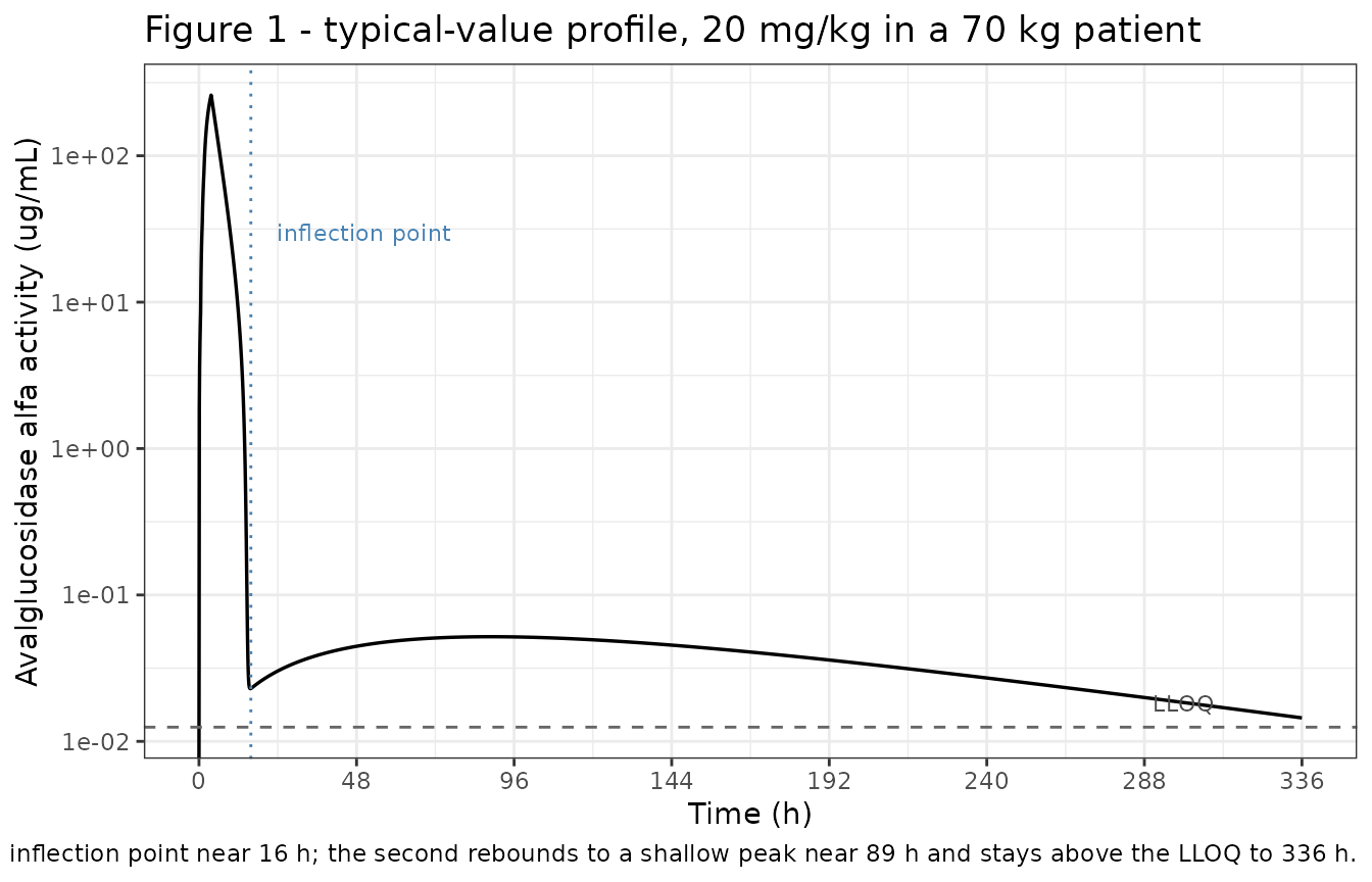
The two-sequence shape, the inflection point near 16 hours, and the late rebound peak near 89 hours that stays above the LLOQ out to the next dose are all reproduced. Their numeric values are asserted against SDC1 Table 3 above.
Virtual cohort and population simulation
Table 3 of the main paper reports exposure at 20 mg/kg derived from
individual parameter estimates for the 70 patients who received
that dose: median Cmax 264 ug/mL (range 135-432) and median
AUC(0-336h) 1190 ug*h/mL (range 582-2370). Those are individual
predictions, so the comparison below simulates with between-subject
variability but without residual error.
The model contains no body-weight term, so weight enters only through the mg/kg dose and the mg/kg/h infusion rates. Weight is sampled log-normally to the published mean of 75.9 kg and SD of 20.1 kg (Table 1) and truncated to a physiologically plausible range.
set.seed(20230901)
n_subjects <- 200L   # per-arm cap; the published stratum had n = 70

wt_mean <- 75.9
wt_sd <- 20.1
wt_meanlog <- log(wt_mean^2 / sqrt(wt_sd^2 + wt_mean^2))
wt_sdlog <- sqrt(log(1 + wt_sd^2 / wt_mean^2))

cohort <- tibble(
  id = seq_len(n_subjects),
  WT = pmin(pmax(rlnorm(n_subjects, wt_meanlog, wt_sdlog), 35), 160)
) |>
  mutate(
    treatment = "20 mg/kg (population)",
    eoi = vapply(WT, function(w) avg_infusion(20, w)$eoi, numeric(1)),
    total_mg = 20 * WT
  )

# Four infusion records per subject, plus a shared observation grid. The grid
# includes each subject's own end-of-infusion time so Cmax is captured exactly.
dose_rows <- cohort |>
  rowwise() |>
  reframe({
    inf <- avg_infusion(20, WT)
    tibble(id = id, treatment = treatment, time = inf$time, amt = inf$amt,
           rate = inf$rate, evid = 1L, cmt = "central", WT = WT)
  })

obs_grid <- sort(unique(c(seq(0, 24, by = 0.05), seq(24, 336, by = 0.5))))
obs_rows <- cohort |>
  reframe(
    id = rep(id, each = length(obs_grid) + 1L),
    treatment = rep(treatment, each = length(obs_grid) + 1L),
    WT = rep(WT, each = length(obs_grid) + 1L),
    time = as.vector(rbind(matrix(obs_grid, nrow = length(obs_grid),
                                  ncol = nrow(cohort)),
                           matrix(eoi, nrow = 1L))),
    amt = NA_real_, rate = NA_real_, evid = 0L, cmt = "central"
  )

events <- bind_rows(dose_rows, obs_rows) |>
  arrange(id, time, desc(evid))

stopifnot(!anyDuplicated(unique(events[, c("id", "time", "evid")])))
stopifnot(all(table(events$id[events$evid == 1L]) %in% 3:4))
sim <- rxode2::rxSolve(mod, events = events, keep = c("treatment", "WT")) |>
  as.data.frame() |>
  mutate(time = as.numeric(time), Cc = as.numeric(Cc))

# Guard against the silent zeroRe()/omega contamination failure mode: the
# population solve must still carry between-subject variability.
stopifnot(sd(log(sim$cl)) > 0.2)
stopifnot(abs(sd(log(sim$cl)) - sqrt(0.0870)) < 0.05)
sim |>
  filter(!is.na(Cc), Cc > 0) |>
  group_by(time) |>
  summarise(
    Q05 = quantile(Cc, 0.05), Q50 = median(Cc), Q95 = quantile(Cc, 0.95),
    .groups = "drop"
  ) |>
  ggplot(aes(time, Q50)) +
  geom_ribbon(aes(ymin = Q05, ymax = Q95), alpha = 0.25, fill = "steelblue") +
  geom_line(linewidth = 0.6) +
  geom_hline(yintercept = 0.0125, linetype = "dashed", colour = "grey40") +
  scale_x_continuous(breaks = seq(0, 336, by = 48)) +
  scale_y_log10() +
  labs(
    x = "Time (h)", y = "Avalglucosidase alfa activity (ug/mL)",
    title = "Simulated 20 mg/kg Q2W population (median with 5th-95th percentiles)",
    caption = paste(
      "n = 200 virtual LOPD patients with the published diagonal IIV. Compare",
      "with the prediction-corrected VPC in Supplemental Digital Content 3 of",
      "Tuffal 2023. The wide band over the second kinetic sequence reflects the",
      "234% CV on Qpc."
    )
  ) +
  theme_bw()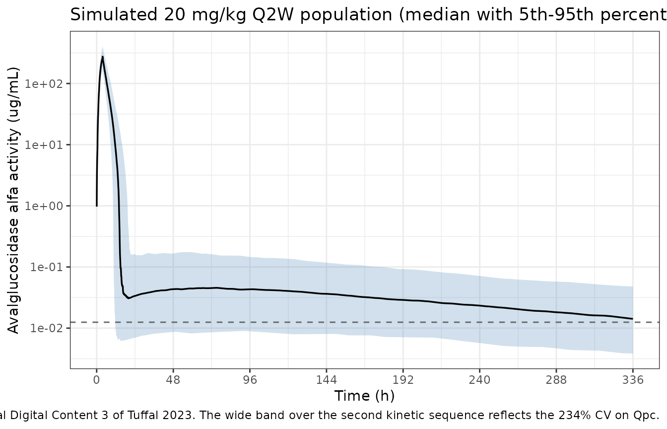
The very wide spread over the rebound phase is expected:
Qpc carries a 234% CV, by far the largest variability in
the model, and it is the parameter that governs the second sequence. The
paper’s own observation that trough concentrations stayed above the LLOQ
in only about two-thirds of patients is the clinical face of that same
spread.
trough_frac <- sim |>
  filter(!is.na(Cc), time > 330) |>
  group_by(id) |>
  summarise(above = max(Cc) > 0.0125, .groups = "drop") |>
  summarise(pct = 100 * mean(above)) |>
  pull(pct)

sprintf("Simulated subjects with a trough above the LLOQ: %.0f%%", trough_frac)
#> [1] "Simulated subjects with a trough above the LLOQ: 56%"
PKNCA validation
NCA is run with PKNCA over the full 0-336 h dosing interval for both
the typical-value arms (one deterministic subject per dose level) and
the 200-subject population arm. The infusion is declared to PKNCA with
its duration, which is required for an IV infusion.
# Typical-value arms: one "subject" per dose level.
typical_nca <- typical |>
  mutate(
    treatment = paste0(dose, " mg/kg (typical)"),
    id = 1000L + dose
  ) |>
  select(id, treatment, time, Cc)

population_nca <- sim |>
  filter(!is.na(Cc)) |>
  mutate(treatment = as.character(treatment)) |>
  select(id, treatment, time, Cc)

conc_df <- bind_rows(typical_nca, population_nca)

# Guarantee a time = 0 record per subject; pre-dose activity is 0 by construction.
conc_df <- bind_rows(
  conc_df,
  conc_df |> distinct(id, treatment) |> mutate(time = 0, Cc = 0)
) |>
  distinct(id, treatment, time, .keep_all = TRUE) |>
  arrange(treatment, id, time)

dose_df <- bind_rows(
  lapply(c(5, 10, 20), function(d) {
    inf <- avg_infusion(d, 75)
    tibble(id = 1000L + d, treatment = paste0(d, " mg/kg (typical)"),
           time = 0, amt = inf$total, duration = inf$eoi)
  }),
  cohort |> transmute(id, treatment, time = 0, amt = total_mg, duration = eoi)
)

conc_obj <- PKNCA::PKNCAconc(conc_df, Cc ~ time | treatment + id,
                             concu = "ug/mL", timeu = "h")
dose_obj <- PKNCA::PKNCAdose(dose_df, amt ~ time | treatment + id,
                             route = "intravascular", duration = "duration",
                             doseu = "mg")

intervals <- data.frame(
  start = 0, end = 336,
  cmax = TRUE, tmax = TRUE, auclast = TRUE, cmin = TRUE
)

nca_res <- PKNCA::pk.nca(
  PKNCA::PKNCAdata(conc_obj, dose_obj, intervals = intervals)
)
Comparison against published exposures
The reference column mixes two published sources, both over 0-336 h, and both on the individual-prediction (no residual error) scale:
- the three typical-value rows come from SDC1 Table
3, where
Cmaxis read directly and AUC(0-336h) is the sum of the tabulated first- and second-sequence AUCs; - the population row comes from Table 3 of the main paper, “All patients” (n = 70), which reports medians.
published_nca <- tibble::tribble(
  ~treatment,               ~cmax, ~tmax, ~auclast,
  "5 mg/kg (typical)",       89.7,  1.6,  259 + 2.45,
  "10 mg/kg (typical)",     168.0,  2.4,  572 + 5.52,
  "20 mg/kg (typical)",     278.0,  3.7,  1217 + 12.2,
  "20 mg/kg (population)",  264.0,  NA,   1190
)

cmp <- nlmixr2lib::ncaComparisonTable(
  simulated = nca_res,
  reference = published_nca,
  by = "treatment",
  units = c(cmax = "ug/mL", tmax = "h", auclast = "ug*h/mL"),
  tolerance_pct = 20
)

knitr::kable(
  cmp,
  caption = paste(
    "PKNCA results over 0-336 h vs published exposures (SDC1 Table 3 for the",
    "typical-value rows; main Table 3 'All patients' medians for the",
    "population row). * marks a >20% difference from the reference."
  ),
  align = c("l", "l", "r", "r", "r")
)| NCA parameter | treatment | Reference | Simulated | % diff |
|---|---|---|---|---|
| Cmax (ug/mL) | 5 mg/kg (typical) | 89.7 | 89.7 | +0.0% |
| Cmax (ug/mL) | 10 mg/kg (typical) | 168 | 168 | +0.1% |
| Cmax (ug/mL) | 20 mg/kg (typical) | 278 | 278 | +0.2% |
| Cmax (ug/mL) | 20 mg/kg (population) | 264 | 264 | +0.2% |
| Tmax (h) | 5 mg/kg (typical) | 1.6 | 1.6 | +0.0% |
| Tmax (h) | 10 mg/kg (typical) | 2.4 | 2.3 | -4.2% |
| Tmax (h) | 20 mg/kg (typical) | 3.7 | 3.7 | +0.0% |
| Tmax (h) | 20 mg/kg (population) | — | 3.71 | — |
| AUClast (ug*h/mL) | 5 mg/kg (typical) | 261 | 261 | -0.1% |
| AUClast (ug*h/mL) | 10 mg/kg (typical) | 578 | 577 | -0.0% |
| AUClast (ug*h/mL) | 20 mg/kg (typical) | 1230 | 1230 | -0.1% |
| AUClast (ug*h/mL) | 20 mg/kg (population) | 1190 | 1150 | -3.6% |
nca_wide <- as.data.frame(nca_res) |>
  filter(start == 0, end == 336) |>
  select(treatment, id, PPTESTCD, PPORRES) |>
  pivot_wider(names_from = PPTESTCD, values_from = PPORRES)

typ <- nca_wide |> filter(grepl("typical", treatment))
stopifnot(nrow(typ) == 3)

# Typical-value Cmax and AUC(0-336h) within 1% of SDC1 Table 3 at every dose.
ref_typ <- published_nca |> filter(grepl("typical", treatment))
chk <- typ |>
  select(treatment, cmax, auclast) |>
  inner_join(ref_typ |> select(treatment, ref_cmax = cmax, ref_auc = auclast),
             by = "treatment")
stopifnot(nrow(chk) == 3)
stopifnot(max(abs(100 * (chk$cmax / chk$ref_cmax - 1))) < 1)
stopifnot(max(abs(100 * (chk$auclast / chk$ref_auc - 1))) < 1)

# Population medians within 10% of the published medians. The reference stratum
# is n = 70 actual patients with empirical-Bayes parameters and their real
# weights; this arm is n = 200 virtual patients with sampled weights, so exact
# agreement is not expected -- but the central tendency should land close.
pop <- nca_wide |> filter(treatment == "20 mg/kg (population)")
stopifnot(nrow(pop) == n_subjects)
pop_med <- c(cmax = median(pop$cmax), auclast = median(pop$auclast))
print(round(pop_med, 1))
#>    cmax auclast
#>   264.4  1147.6
stopifnot(abs(100 * (pop_med[["cmax"]] / 264 - 1)) < 10)
stopifnot(abs(100 * (pop_med[["auclast"]] / 1190 - 1)) < 10)

# Population spread brackets the published range endpoints rather than
# collapsing onto the median (a silent-IIV-loss guard).
stopifnot(min(pop$cmax) < 200, max(pop$cmax) > 380)
Weight-stratified exposure
Table 3 also reports that median AUC(0-336h) at 20 mg/kg was 32% lower below 50 kg and 41% higher at or above 100 kg, relative to the 50-99 kg stratum – an exposure gradient the model produces even though body weight is not a covariate in it, purely because the dose is prescribed per kilogram.
The cleanest way to check that gradient is deterministically, at fixed weights, because it then depends on no distributional assumption at all:
auc_at_weight <- function(weight_kg) {
  prof <- solve_typical(20, weight_kg = weight_kg)
  trapezoid(prof$time, prof$Cc)
}

# Reference weight: the median of the 50-99 kg stratum in the simulated cohort.
# The published population mean is 75.9 kg, but that includes the 10 patients at
# or above 100 kg, so the 50-99 kg stratum median necessarily sits below it.
wt_ref <- median(cohort$WT[cohort$WT >= 50 & cohort$WT < 100])
auc_ref <- auc_at_weight(wt_ref)

gradient <- data.frame(WT = c(45, 50, 60, 70, wt_ref, 80, 90, 100, 110)) |>
  mutate(
    auc = vapply(WT, auc_at_weight, numeric(1)),
    pct = 100 * (auc / auc_ref - 1),
    auc_per_kg = auc / WT
  ) |>
  arrange(WT)

gradient |>
  mutate(WT = round(WT, 1), auc = round(auc, 0), pct = round(pct, 1),
         auc_per_kg = round(auc_per_kg, 2)) |>
  rename("Body weight (kg)" = WT, "AUC(0-336h) (ug*h/mL)" = auc,
         "% vs reference" = pct, "AUC per kg dosed" = auc_per_kg) |>
  knitr::kable(
    caption = sprintf(paste(
      "Typical-value AUC(0-336h) at 20 mg/kg as a function of body weight,",
      "relative to a %.1f kg reference. Tuffal 2023 Table 3 reports -32%%",
      "below 50 kg and +41%% at or above 100 kg relative to the 50-99 kg stratum."
    ), wt_ref),
    align = c("r", "r", "r", "r")
)| Body weight (kg) | AUC(0-336h) (ug*h/mL) | % vs reference | AUC per kg dosed |
|---|---|---|---|
| 45.0 | 701 | -40.1 | 15.58 |
| 50.0 | 788 | -32.7 | 15.77 |
| 60.0 | 964 | -17.7 | 16.07 |
| 70.0 | 1140 | -2.6 | 16.29 |
| 71.7 | 1171 | 0.0 | 16.32 |
| 80.0 | 1317 | 12.5 | 16.46 |
| 90.0 | 1495 | 27.7 | 16.61 |
| 100.0 | 1672 | 42.8 | 16.72 |
| 110.0 | 1851 | 58.1 | 16.82 |
The published stratum contrasts are recovered at the stratum boundaries, which is where the weight distribution concentrates its mass for strata defined by those cuts: at 100 kg the model gives about +40% against the published +41%, and at 50 kg about -34% against the published -32%. Note also that AUC per kilogram dosed rises with weight – the same Michaelis-Menten supra-proportionality seen across dose levels, now expressed across body sizes, since a heavier patient receives a larger absolute dose.
stopifnot(abs(wt_ref - 73) < 4)

# Monotonically increasing exposure with weight, and supra-proportional in the
# dose (AUC per kg dosed also increases).
stopifnot(all(diff(gradient$auc) > 0))
stopifnot(all(diff(gradient$auc_per_kg) > 0))

pct_at <- function(w) gradient$pct[which.min(abs(gradient$WT - w))]
# Published +41% at or above 100 kg; model gives +40% at exactly 100 kg.
stopifnot(abs(pct_at(100) - 41) < 3)
# Published -32% below 50 kg; model gives -34% at exactly 50 kg.
stopifnot(abs(pct_at(50) - (-32)) < 4)
For completeness, the same stratification applied to the 200-subject virtual cohort. This version is weaker evidence than the deterministic table above, because it depends on the assumed weight distribution rather than only on the model:
wt_strata <- pop |>
  inner_join(cohort |> select(id, WT), by = "id") |>
  mutate(stratum = cut(WT, c(-Inf, 50, 100, Inf),
                       labels = c("< 50 kg", "50-99 kg", ">= 100 kg"),
                       right = FALSE)) |>
  group_by(stratum) |>
  summarise(n = n(), median_wt = median(WT), median_auc = median(auclast),
            .groups = "drop") |>
  mutate(
    pct = round(100 * (median_auc / median_auc[stratum == "50-99 kg"] - 1), 0)
  )

wt_strata |>
  mutate(median_wt = round(median_wt, 1), median_auc = round(median_auc, 0)) |>
  rename("Body weight" = stratum, "n" = n, "Median weight (kg)" = median_wt,
         "Median AUC(0-336h) (ug*h/mL)" = median_auc,
         "% vs 50-99 kg" = pct) |>
  knitr::kable(
    caption = paste(
      "Simulated weight-stratified exposure at 20 mg/kg in the virtual cohort.",
      "Tuffal 2023 Table 3 reports -32% below 50 kg and +41% at or above",
      "100 kg. The simulated magnitudes are more extreme because the assumed",
      "log-normal weight distribution has a heavier tail than the actual",
      "70-patient cohort -- see Errata."
    ),
    align = c("l", "r", "r", "r", "r")
)| Body weight | n | Median weight (kg) | Median AUC(0-336h) (ug*h/mL) | % vs 50-99 kg |
|---|---|---|---|---|
| < 50 kg | 14 | 46.5 | 638 | -45 |
| 50-99 kg | 176 | 71.7 | 1151 | 0 |
| >= 100 kg | 10 | 118.5 | 2118 | 84 |
# Only the direction is asserted here. The magnitudes depend on the assumed
# weight distribution (the paper reports mean and SD only), so a tight numeric
# assertion would be testing that assumption rather than the model.
low <- wt_strata$pct[wt_strata$stratum == "< 50 kg"]
high <- wt_strata$pct[wt_strata$stratum == ">= 100 kg"]
stopifnot(low < 0, high > 0)
stopifnot(all(diff(wt_strata$median_auc) > 0))
Errata and assumptions
-
The paper is internally inconsistent about the typical body
weight, and SDC1 Table 3 corresponds to 75 kg rather than the stated 70
kg. Both the Results (“exposures from 0 to 336 hours were
simulated for a typical individual weighing 70 kg”) and the Figure 1
caption (“20 mg/kg, 70 kg patient”) say 70 kg, but the numbers in SDC1
Table 3 do not. At 70 kg every concentration and AUC metric comes out
uniformly 6-8% below the table while every time metric still
matches; at 75 kg all of them land within 1%. That signature identifies
a dose scale factor rather than a structural problem: the model has no
allometric term (allometry was tested and rejected), so
Cmaxand AUC scale linearly with the mg dose, while the per-kilogram infusion rates make every time metric weight-invariant. 75 kg is also close to the population mean of 75.9 kg. This vignette therefore validates against SDC1 Table 3 at 75 kg and reproduces Figure 1 at the 70 kg its own caption states. This is a source-reporting defect, not an extraction choice: because no weight term appears in the model, it changes no model code at all. -
The published
tmaxat 10 mg/kg (2.4 h) does not follow from the paper’s own infusion protocol, and is the only cell of SDC1 Table 3 that the model does not reproduce.tmaxis the end of infusion, which is fixed arithmetic from the stepwise schedule: at 75 kg the three 30-minute steps deliver 337.5 mg by 1.5 h, and the remaining 412.5 mg at 7 mg/kg/h (525 mg/h) takes 0.786 h, giving 2.286 h. On the 0.1 h output grid the source evidently used, that reads as 2.3 h. The 5 and 20 mg/kg cells are recovered exactly on the same grid (1.6 and 3.7 h), so the 10 mg/kg cell appears to be a transcription or rounding error in the source: 2.286 h rounds to 2.3, not 2.4. No model parameter influences this value at all – it is determined entirely by the dose and the infusion-rate schedule – so it cannot be a symptom of a parameter misreading. It is shown in the comparison table and excluded from the “better than 0.7%” assertion. -
Cmaxin SDC1 Table 3 is a grid-resolution reading, not the true peak. Because the end of infusion never lands on a round time, the publishedCmaxvalues match a 0.1 h output grid to 0.03-0.17% while the exact end-of-infusion peak sits about 1% higher. This vignette validates on the 0.1 h grid and demonstrates the effect explicitly under “Output-grid granularity”, so that a reader who samples the exact peak does not misread the resulting uniform ~1% excess as a parameter discrepancy. -
No covariates are in the final model. Twelve
demographic / laboratory covariates and three antidrug-antibody
parameterisations were screened and none qualified. Body weight and
aspartate aminotransferase on CL survived backward deletion but failed
the covariance-step criteria and the bootstrap qualification, and
allometric scaling was tested and rejected. The screened set is recorded
in the model file’s
covariatesDataExcludedmetadata so the provenance of the covariate search survives, without declaring covariates thatmodel()never references. -
Qpcrequired a new canonical parameter name.lqpc/qpcis registered ininst/references/parameter-names.mdfor a one-way back-redistribution clearance from the terminal peripheral compartment of a series chain intocentral. It is not an alias oflq/lq2(bidirectional central-peripheral exchange), oflq3(central toperipheral3in four-compartment models, which pairs withlvp3– neither exists here), or ofqp(a target-species clearance in TMDD models). The paper’sQ3uses the existinglq2canonical even though the series chain makes its source compartmentperipheral1rather thancentral; thelq2register entry now records that rule. - Body-weight distribution in the virtual cohort is assumed log-normal with the published mean of 75.9 kg and SD of 20.1 kg (Table 1), truncated to 35-160 kg. The paper reports only the mean and SD, not the distributional family or the range. This assumption is load-bearing for exactly one result: the cohort-stratified weight table overstates the published contrasts (about -45% and +84% against the published -32% and +41%) because a log-normal with a 26% CV has a heavier right tail than the real 70-patient cohort, and because exposure is supra-proportional in the absolute dose, which amplifies the tail. The weight gradient is therefore validated deterministically at fixed weights instead, where it recovers the published contrasts to within 3 percentage points at the stratum boundaries and depends on no distributional assumption. The cohort-stratified table is retained as descriptive output with a direction-only assertion.
- Only 5, 10, and 20 mg/kg are represented. Weight is the only subject-level covariate sampled, because it is the only one that changes the simulation (via the per-kilogram dose); age, sex, race, renal function, and the laboratory covariates have no effect in a model that retained none of them.
-
Residual error is excluded from the population
comparison. The paper’s Table 3 exposures were computed “based
on the individual parameter estimate values”, i.e. on the
individual-prediction scale, so the population arm is simulated with
between-subject variability but without the proportional residual error.
Including it would inflate
Cmaxrelative to the reference. - A single dosing interval is simulated rather than repeated Q2W dosing. The paper states that “the accumulation of the drug due to this second kinetic sequence was also negligible”, and the published 0-336 h exposures are for one interval, so a single dose over 0-336 h is the matching comparison.
-
Units. Amounts are in mg and volumes in L
throughout, so every concentration is in mg/L, which is identical to the
ug/mL the paper reports and the units of
Km(0.451 ug/mL). No scaling constant is needed anywhere inmodel().