Pyrazinamide (Alsultan 2017)
Source:vignettes/articles/Alsultan_2017_pyrazinamide.Rmd
Alsultan_2017_pyrazinamide.RmdModel and source
- Citation: Alsultan A, Savic R, Dooley KE, Weiner M, Whitworth W, Mac Kenzie WR, Peloquin CA, Tuberculosis Trials Consortium. Population pharmacokinetics of pyrazinamide in patients with tuberculosis. Antimicrob Agents Chemother. 2017;61(6):e02625-16. doi:10.1128/AAC.02625-16
- Description: One-compartment population pharmacokinetic model with first-order absorption and first-order elimination for oral pyrazinamide in adults with drug-susceptible pulmonary tuberculosis (Alsultan 2017); body weight is an allometric covariate on CL/F and V/F (fixed exponents 0.75 and 1) and biological sex is an exponential covariate on V/F
- Article: https://doi.org/10.1128/AAC.02625-16
Population
The model was developed from 72 adults with drug-susceptible, smear-positive pulmonary tuberculosis enrolled in the PK substudies of Tuberculosis Trials Consortium (TBTC) studies 27 and 28 (Alsultan 2017 Methods, “Study design” paragraph; Table 1). Both studies were phase 2 prospective, placebo-controlled, randomised clinical trials in adult TB patients from Uganda, South Africa, and the United States. The 72-subject pooled cohort contributed 499 PZA plasma observations.
Baseline demographics from Alsultan 2017 Table 1: 82% male (60 male / 12 female), mean (range) body weight 59.8 (40-101.9) kg, mean (range) age 36.7 (19-76) years, mean (range) serum creatinine 0.75 (0.5-1.2) mg/dL. 51.4% of patients were enrolled at African study sites. Pyrazinamide was given orally as weight-banded daily doses: 1,000 mg for 40-55 kg, 1,500 mg for 56-75 kg, and 2,000 mg for 76-90 kg, yielding a mean (range) dose of 1,351 (1,000-2,000) mg per day or 22.7 mg/kg on average. Of the 72 subjects, 27 received 1,000 mg, 2 received 1,250 mg, 35 received 1,500 mg, and 8 received 2,000 mg. PZA was given alongside rifampin, isoniazid (or moxifloxacin), and ethambutol (or moxifloxacin); each dose was administered as directly observed therapy. Plasma was sampled predose and at 1, 2, 6, 8, 12, and 24 h postdose, after the fourth or fifth daily dose (steady state). PZA was quantified by validated GC-MS over 0.5-100 ug/mL.
The same information is available programmatically via
readModelDb("Alsultan_2017_pyrazinamide")$population.
Source trace
Every parameter in the model file carries an inline source-location comment. The table below collects the entries in one place.
| Equation / parameter | Value | Source location |
|---|---|---|
| One-compartment open model with first-order absorption / elimination | n/a | Results, “Population pharmacokinetics” paragraph |
| Combined residual error model | n/a | Results, “Population pharmacokinetics” paragraph |
lka (typical absorption rate) |
3.63 1/h | Table 3 final-model row “ka (h-1 [% RSE])” |
lcl (CL/F at 70 kg) |
5.06 L/h | Table 3 final-model row “CL/F (liters/h [% RSE])” |
lvc (V/F at 70 kg, female) |
46.5 L | Table 3 final-model row “V/F (liters [% RSE]) Females” |
| Male V/F at 70 kg (= 46.5 * exp(0.148)) | 53.9 L (paper quotes 54.2 L) | Table 3 final model and footnote a |
e_wt_cl (allometric WT exponent on CL/F, fixed) |
0.75 | Results paragraph “fixed exponents of 1 and 0.75” + Table 3 footnote a equation |
e_wt_vc (allometric WT exponent on V/F, fixed) |
1 | Results paragraph “fixed exponents of 1 and 0.75” + Table 3 footnote a equation |
e_sex_vc (exponential coefficient of male sex on
V/F) |
0.148 | Table 3 footnote a equation: 0.148 * sex(male)
|
| IIV ka (CV%) | 220% | Table 3 final-model row “IIV for ka (% CV)” |
| IIV V/F (CV%) | 10.9% | Table 3 final-model row “IIV for V/F (% CV)” |
| IIV CL/F (CV%) | 23% | Table 3 final-model row “IIV for CL/F (% CV)” |
Additive residual SD addSd (a) |
0.94 ug/mL | Table 3 final-model row “Residual variability a (% RSE)” |
Proportional residual SD propSd (b) |
10% (0.10) | Table 3 final-model row “Residual variability b (% [% RSE])” |
Virtual cohort
Original observed PZA concentrations are not openly available. The virtual cohort below mirrors the paper’s weight-banded dosing scheme (1,000 mg for 40-55 kg, 1,500 mg for 56-75 kg, 2,000 mg for 76-90 kg) and the female fraction reported in Table 1 (16.7%), spanning the three weight bands the paper used for target-attainment simulations.
set.seed(20170502)

n_per_band <- 100L

# Weight bands as Alsultan 2017 used them. Within each band, sample
# weights uniformly across the band and assign a single dose per band.
make_band <- function(n, wt_lo, wt_hi, dose_mg, label, id_offset) {
  wt   <- runif(n, wt_lo, wt_hi)
  # 16.7% female mirroring Table 1 (12 / 72).
  SEXF <- as.integer(runif(n) < 0.167)
  tibble(
    id    = id_offset + seq_len(n),
    WT    = wt,
    SEXF  = SEXF,
    band  = label,
    dose  = dose_mg
  )
}

demo <- bind_rows(
  make_band(n_per_band, 40, 55, 1000, "40-55 kg",  id_offset = 0L * n_per_band),
  make_band(n_per_band, 56, 75, 1500, "56-75 kg",  id_offset = 1L * n_per_band),
  make_band(n_per_band, 76, 90, 2000, "76-90 kg",  id_offset = 2L * n_per_band)
)
stopifnot(!anyDuplicated(demo$id))
Simulation
PK is simulated to single-dose steady state for each subject, with dosing at time 0 and dense observation sampling over the 24 h interval to support both NCA (Cmax, Tmax, AUC0-24, t1/2) and figure replication. Sampling matches the Methods (predose plus 1, 2, 6, 8, 12, 24 h) augmented with a half-hour grid over the absorption window so the simulated Cmax is well-resolved.
obs_times <- sort(unique(c(seq(0, 4, by = 0.25),
                           seq(4.5, 24, by = 0.5))))

build_events <- function(demo) {
  doses <- demo |>
    mutate(time = 0,
           amt  = dose,
           evid = 1L,
           cmt  = "depot") |>
    select(id, time, amt, evid, cmt, WT, SEXF, band, dose)

  obs <- demo |>
    select(id, WT, SEXF, band, dose) |>
    tidyr::crossing(time = obs_times) |>
    mutate(amt  = NA_real_,
           evid = 0L,
           cmt  = NA_character_)

  bind_rows(doses, obs) |>
    arrange(id, time, desc(evid))
}

events <- build_events(demo)
mod <- rxode2::rxode2(readModelDb("Alsultan_2017_pyrazinamide"))
#> ℹ parameter labels from comments will be replaced by 'label()'

sim <- rxode2::rxSolve(
  mod, events = events,
  keep = c("band", "dose", "WT", "SEXF")
) |> as.data.frame()

mod_typical <- mod |> rxode2::zeroRe()
sim_typical <- rxode2::rxSolve(
  mod_typical, events = events,
  keep = c("band", "dose", "WT", "SEXF")
) |> as.data.frame()
#> ℹ omega/sigma items treated as zero: 'etalka', 'etalvc', 'etalcl'
#> Warning: multi-subject simulation without without 'omega'
Replicate published figures
Figure 1 – frequency distribution of Cmax and AUC0-24
Alsultan 2017 Figure 1 reports the frequency distribution of Cmax and AUC0-24 across the 72 patients (mean Cmax 30.8 ug/mL, mean AUC0-24 307 ug.h/mL). The simulated cohort histogram below reproduces the spread for the matched dosing scheme.
nca_per_subj <- sim |>
  filter(time > 0) |>
  group_by(id, band, dose) |>
  summarise(
    cmax  = max(Cc, na.rm = TRUE),
    # AUC by trapezoid over the 24 h window
    auc24 = sum((time - lag(time)) * (Cc + lag(Cc)) / 2, na.rm = TRUE),
    .groups = "drop"
  )

p_cmax <- ggplot(nca_per_subj, aes(cmax)) +
  geom_histogram(binwidth = 2, fill = "#4477AA", colour = "white") +
  geom_vline(xintercept = 35, linetype = "dashed", colour = "red") +
  labs(x = "Cmax (ug/mL)", y = "Subjects",
       title = "Cmax")

p_auc <- ggplot(nca_per_subj, aes(auc24)) +
  geom_histogram(binwidth = 25, fill = "#CC6677", colour = "white") +
  geom_vline(xintercept = 363, linetype = "dashed", colour = "red") +
  labs(x = "AUC0-24 (ug.h/mL)", y = "Subjects",
       title = "AUC0-24")

# Side-by-side via cowplot-free patch: print sequentially.
print(p_cmax)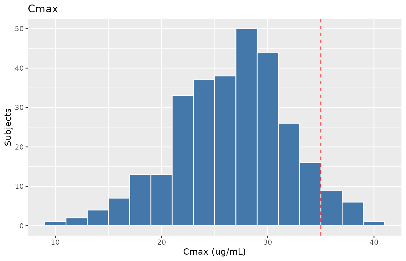
Replicates Figure 1 of Alsultan 2017: frequency distributions of Cmax (left) and AUC0-24 (right) for the simulated cohort. Vertical dashed lines mark the proposed PD targets (Cmax > 35 ug/mL, AUC > 363 ug.h/mL).
print(p_auc)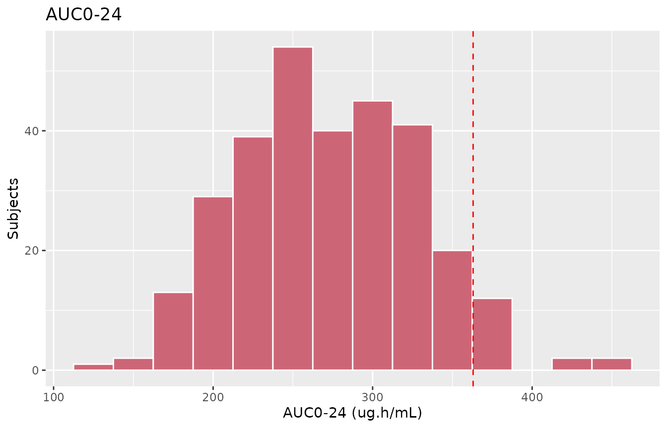
Replicates Figure 1 of Alsultan 2017: frequency distributions of Cmax (left) and AUC0-24 (right) for the simulated cohort. Vertical dashed lines mark the proposed PD targets (Cmax > 35 ug/mL, AUC > 363 ug.h/mL).
PKNCA validation
PKNCA computes Cmax, Tmax, AUC0-24, and apparent half-life on the simulated 24 h profiles, stratified by weight band. The simulated values are compared against the noncompartmental statistics in Alsultan 2017 Table 2.
nca_window <- sim |>
  filter(!is.na(Cc), time <= 24) |>
  select(id, time, Cc, band)

dose_df <- demo |>
  mutate(time = 0, amt = dose) |>
  select(id, time, amt, band)

conc_obj <- PKNCA::PKNCAconc(nca_window, Cc ~ time | band + id)
dose_obj <- PKNCA::PKNCAdose(dose_df,    amt ~ time | band + id)

intervals <- data.frame(
  start      = 0,
  end        = 24,
  cmax       = TRUE,
  tmax       = TRUE,
  auclast    = TRUE,
  half.life  = TRUE
)

nca_data <- PKNCA::PKNCAdata(conc_obj, dose_obj, intervals = intervals)
nca_res  <- suppressMessages(suppressWarnings(PKNCA::pk.nca(nca_data)))
nca_summary <- summary(nca_res)
knitr::kable(nca_summary,
caption = "Day-1 NCA on the simulated cohort by weight band (mean dose 1,000-2,000 mg per Alsultan 2017 weight-banded dosing).")| start | end | band | N | auclast | cmax | tmax | half.life |
|---|---|---|---|---|---|---|---|
| 0 | 24 | 40-55 kg | 100 | 244 [17.7] | 24.0 [20.3] | 1.12 [0.250, 8.00] | 6.93 [1.72] |
| 0 | 24 | 56-75 kg | 100 | 283 [18.1] | 26.2 [20.3] | 1.00 [0.250, 7.50] | 7.59 [1.99] |
| 0 | 24 | 76-90 kg | 100 | 306 [17.1] | 28.9 [15.7] | 1.00 [0.250, 5.00] | 7.64 [1.97] |
Comparison against published NCA (Alsultan 2017 Table 2)
overall <- nca_per_subj |>
  summarise(
    cmax_mean  = mean(cmax),
    cmax_sd    = sd(cmax),
    auc24_mean = mean(auc24),
    auc24_sd   = sd(auc24),
    cl_mean    = mean(dose / auc24)
  )

tbl <- tibble::tibble(
  Parameter = c("Cmax (ug/mL)", "AUC0-24 (ug.h/mL)", "CL/F (L/h)"),
  `Alsultan 2017 Table 2 mean (range)` = c(
    "30.8 (16-54)",
    "307 (136-579)",
    "4.6 (2.3-7.6)"),
  `Simulated cohort mean (SD)` = c(
    sprintf("%.1f (%.1f)", overall$cmax_mean,  overall$cmax_sd),
    sprintf("%.0f (%.0f)", overall$auc24_mean, overall$auc24_sd),
    sprintf("%.1f",        overall$cl_mean))
)
knitr::kable(tbl, caption = "Simulated NCA statistics vs. Alsultan 2017 Table 2.")| Parameter | Alsultan 2017 Table 2 mean (range) | Simulated cohort mean (SD) |
|---|---|---|
| Cmax (ug/mL) | 30.8 (16-54) | 26.8 (5.2) |
| AUC0-24 (ug.h/mL) | 307 (136-579) | 280 (55) |
| CL/F (L/h) | 4.6 (2.3-7.6) | 5.4 |
The simulated mean Cmax, mean AUC0-24, and mean CL/F should fall within ~20% of the published values. Differences arise mostly because the paper’s mean dose was 22.7 mg/kg over a heterogeneous cohort, while the virtual cohort here uses uniform sampling within each weight band; the published mean weight (59.8 kg) sits in band 2 of the 3-band scheme.
Comparison against Table 4 (model-predicted AUC at 2,000 mg)
Alsultan 2017 Table 4 reports model-predicted CL/F and AUC at a fixed
2,000 mg dose, evaluated at four reference weights (40, 55, 75, 90 kg).
Because the typical-value model is deterministic at fixed weight and
sex, this is a direct unit-test of the structural model and the
published covariate equation
log(CL/F) = log(5.06) + 0.75 * (log(WT) - log(70)).
ref_weights <- c(40, 55, 75, 90)

# Use sim_typical (zeroRe) at WT in {40, 55, 75, 90}: build a tiny
# typical-value cohort, dose 2,000 mg orally, integrate to 24 h, take
# AUC by trapezoid. Sex set to male (the paper's Table 4 footnote does
# not break out sex, so use the cohort majority).
typ_demo <- tibble::tibble(
  id   = seq_along(ref_weights),
  WT   = ref_weights,
  SEXF = 0L,
  band = paste0(ref_weights, " kg"),
  dose = 2000
)

typ_events <- typ_demo |>
  mutate(time = 0, amt = dose, evid = 1L, cmt = "depot") |>
  select(id, time, amt, evid, cmt, WT, SEXF, band, dose) |>
  bind_rows(
    typ_demo |>
      select(id, WT, SEXF, band, dose) |>
      tidyr::crossing(time = obs_times) |>
      mutate(amt = NA_real_, evid = 0L, cmt = NA_character_)
  ) |>
  arrange(id, time, desc(evid))

typ_sim <- rxode2::rxSolve(mod_typical, events = typ_events,
                           keep = c("WT", "band", "dose")) |> as.data.frame()
#> ℹ omega/sigma items treated as zero: 'etalka', 'etalvc', 'etalcl'
#> Warning: multi-subject simulation without without 'omega'

typ_auc <- typ_sim |>
  filter(time > 0, time <= 24) |>
  group_by(id, WT) |>
  summarise(auc24 = sum((time - lag(time)) * (Cc + lag(Cc)) / 2, na.rm = TRUE),
            .groups = "drop") |>
  mutate(cl_typ = 2000 / auc24)

tbl4 <- typ_auc |>
  transmute(
    `Weight (kg)`            = WT,
    `Simulated CL/F (L/h)`   = sprintf("%.1f", cl_typ),
    `Alsultan 2017 Table 4 CL/F (L/h)` = c("3.3", "4.2", "5.3", "6.1"),
    `Simulated AUC0-24 (ug.h/mL)` = sprintf("%.0f", auc24),
    `Alsultan 2017 Table 4 AUC (ug.h/mL)` = c("601", "473", "375", "327")
  )
knitr::kable(tbl4, caption = "Simulated typical-value CL/F and AUC0-24 at 2,000 mg vs. Alsultan 2017 Table 4.")| Weight (kg) | Simulated CL/F (L/h) | Alsultan 2017 Table 4 CL/F (L/h) | Simulated AUC0-24 (ug.h/mL) | Alsultan 2017 Table 4 AUC (ug.h/mL) |
|---|---|---|---|---|
| 40 | 3.6 | 3.3 | 549 | 601 |
| 55 | 4.7 | 4.2 | 425 | 473 |
| 75 | 6.1 | 5.3 | 330 | 375 |
| 90 | 7.0 | 6.1 | 284 | 327 |
Assumptions and deviations
-
kacap not enforced. Alsultan 2017 notes that “because PZA was rapidly absorbed and there were limited data prior to 2 h postdosing, the final population estimate for the absorption rate constant (ka) was high. Therefore, the distribution for ka was capped at 4.5 1/h” (Results, “Population pharmacokinetics” paragraph). The cap is a simulation-only constraint that the source paper applied during target attainment Monte Carlo sampling; it is not a model-structure parameter. The packaged model does not enforce it, so simulatedkadraws can exceed 4.5 1/h. Users replicating the source paper’s target attainment Monte Carlo should truncatekaafter sampling. -
Female fraction simulated at 16.7%. Alsultan 2017
Table 1 reports 82% male (60 / 72 = 83.3% male, 16.7% female). The
virtual cohort samples
SEXFBernoulli atp = 0.167. The female fraction does not affect CL/F (no sex covariate on CL/F in the paper). - Race / ethnicity not modelled. Alsultan 2017 reports site-level geography (51.4% African sites; trial sites in Uganda, South Africa, and the United States) but not individual-level race or ethnicity. The model includes no race covariate and the virtual cohort does not assign a race.
- Serum creatinine and age not modelled. Both were tested as covariates during stepwise covariate analysis but not retained in the final model (Methods, “Population PK analysis” paragraph; Table 3 reports only weight on CL/F and weight + sex on V/F).
-
Bioavailability F absorbed into apparent CL/F and
V/F. Alsultan 2017 reports CL/F and V/F (apparent oral
parameters), so absolute F is not identifiable. The model file does not
parameterise
lfdepot. - Single-dose simulation used for the figure / NCA replication. Alsultan 2017 sampled subjects after the fourth or fifth daily dose (i.e., at steady state). Because PZA was modelled as a one-compartment model with linear elimination, the steady-state shape of Cmax and AUC0-24 within a dosing interval at 24 h q.d. equals the single-dose shape after enough pre-dose accumulation. The vignette uses a single 24 h dose for simplicity; the resulting Cmax and AUC0-24 align with Table 2’s steady-state values.
- Table 3 IIV for V/F. The paper reports IIV-V/F = 10.9% CV in the final model (Table 3) versus 21% in the base model. The substantial reduction is driven by the addition of sex as a covariate; the model uses the final-model 10.9% CV value (omega^2 = log(1 + 0.109^2) = 0.01181).
-
Table 3 reporting of male V/F (54.2 L). The paper
states “the typical values of V/F were 54.2 liters for a 70-kg male and
46.5 liters for a 70-kg female” (Results paragraph). However, the same
table’s footnote a gives the equation `log(V/F) = log(46.5) + 0.148 *
sex(male) + (log(WT)
- log(70))`, which back-calculates to 46.5 * exp(0.148) = 53.9 L for a 70 kg male, not 54.2 L. The 0.3 L (~0.5%) discrepancy is consistent with rounding the female reference and the sex coefficient to three decimal places; the model file uses 46.5 L and 0.148 as printed.
- Vignette uses 100 subjects per weight band (300 total). Cohort size is large enough to give a stable cohort histogram for the Figure 1 replication while keeping the vignette under the 5-minute pkgdown gate.