Somatrogon (Wang 2025)

Model and source

Citation: Wang Y, Pei X, Niu T, Korth-Bradley J, Fostvedt L. Implementing a Bayesian approach using Stan with Torsten: Population pharmacokinetics analysis of somatrogon. CPT Pharmacometrics Syst Pharmacol. 2025;14(2):351-364. doi:10.1002/psp4.13279
Description: Two-compartment population PK model with delayed first-order absorption for somatrogon in children with growth hormone deficiency, estimated by fully Bayesian MCMC (Stan/Torsten) (Wang 2025)
Article: https://doi.org/10.1002/psp4.13279
Supplement (Data S1-S9, including the Stan model files and the NONMEM control stream used below to resolve the allometric normalizer): https://www.ebi.ac.uk/europepmc/webservices/rest/PMC11812939/supplementaryFiles

Somatrogon (NGENLA) is a recombinant long-acting growth hormone given as a once-weekly subcutaneous injection for growth hormone deficiency (GHD) in children from 3 years of age. Wang 2025 re-estimates the somatrogon population PK model with a fully Bayesian approach – Stan with the Torsten package – rather than the first-order conditional estimation with interaction (FOCEI) method used for the previously published NONMEM analyses.

This is a methods paper, but it is not a review: the authors fit their own model, to their own data, and report their own posterior estimates. It is that fitted model which is packaged here.

Why this model is worth having separately

The previously published “Phase III PopPK model” estimated the effect of time-varying anti-drug antibody status (ADAT) on apparent clearance while fixing most other PK parameters to the Phase II estimates. As Wang 2025 puts it, that approach ignores the uncertainty in the fixed parameters, which propagates into every prediction made from the model. The Bayesian re-analysis estimates all parameters jointly, including a full 4x4 covariance matrix across the random effects, where the earlier analyses had assumed independence.

Population

The packaged parameters were estimated from the 560 observations of the 42 pediatric participants of the Phase II study CP-4-004 (Wang 2025, Results, first paragraph). Baseline demographics are Wang 2025 Table 3, column “Phase II (004)”: median body weight 14.8 kg (range 10-26.3), median age 5.5 years (range 3-11), 33.3% female, 95.2% White. Weekly doses ranged 3.05-17.5 mg (0.228-0.711 mg/kg/week), median 6.74 mg/week.

Two inclusion details matter for interpreting the parameters:

Although Study 004 followed participants for up to 5.5 years, only PK samples collected within 1 year of study start were used, to reduce MCMC run time (Methods, “Data inclusion criteria”).
The 109 pediatric participants of the Phase III study CP-4-006 were not used for estimation. They served only as an external set for posterior prediction (Table 2), so their demographics are not reflected in these parameters.

str(readModelDb("Wang_2025_somatrogon")()$population)
#> List of 14
#>  $ species       : chr "human"
#>  $ n_subjects    : num 42
#>  $ n_studies     : num 1
#>  $ n_observations: num 560
#>  $ age_range     : chr "3-11 years"
#>  $ age_median    : chr "5.5 years"
#>  $ weight_range  : chr "10-26.3 kg"
#>  $ weight_median : chr "14.8 kg"
#>  $ sex_female_pct: num 33.3
#>  $ race_ethnicity: Named num [1:3] 95.2 2.4 2.4
#>   ..- attr(*, "names")= chr [1:3] "White" "African American" "Other or Missing"
#>  $ disease_state : chr "Pediatric growth hormone deficiency (GHD)"
#>  $ dose_range    : chr "3.05-17.5 mg/week (0.228-0.711 mg/kg/week) by once-weekly subcutaneous injection; median 6.74 mg/week (0.482 mg/kg/week)"
#>  $ regions       : chr "Not reported in the article"
#>  $ notes         : chr "Baseline demographics from Wang 2025 Table 3, column 'Phase II (004)'. Posterior sampling used the 560 observat"| __truncated__

Model structure

A two-compartment model with delayed first-order absorption. All disposition parameters are apparent (/F): bioavailability was fixed to 1 in the pediatric data (Data S3 F1 = THETA(7)*FPROT with THETA(7) = 1 FIX; Data S5 F[1] = 1), so no lfdepot is estimable and none is carried.

Three structural features are worth calling out because the article’s prose understates them; all three were confirmed against the Stan model file shipped as Data S5.

1. The allometric exponents are estimated and shared pairwise. A single exponent e_wt_cl_q = 1.258 applies to both CL/F and Q/F, and a single e_wt_vc_vp = 1.341 applies to both Vc/F and Vp/F – exactly as Table 5 labels its rows (“Weight effect on CL/F and Q/F”, “Weight effect on Vc/F and Vp/F”) and as Data S5 applies thetaWT1 and thetaWT2. Neither is fixed at the 0.75/1 allometric convention, and both exceed it substantially.

2. The allometric normalizer is 15 kg, and it is not printed in the article. In Data S5 the weight term enters pre-computed as a data column (WTrt), so neither the article nor the Stan code discloses the reference value. It is recoverable from the NONMEM control stream shipped as Data S3:

;;; CLBWT-DEFINITION START  MEDIAN BWT = 14.8 in pediatric patients
    CLBWT = ((WT/15)**THETA(9))  ;;; 15 is the median body weight for study 004

i.e. the Study 004 median weight of 14.8 kg (Table 3), rounded to 15. Note that the normalizer (15) and the reported cohort median (14.8) are not the same number; the model file uses 15, per the control stream.

3. The ADA effect carries its own gated random effect. ADA-positive occasions get both a proportional shift in CL/F and an additional between-subject random effect on CL/F. In Data S5 both sit inside one branch:

if (ADAT[i] == 1 && ADAS[i] == 1) {
  theta[i,1] = CLHat*(WTrt[i]^thetaWT1)*(1+thetaAD)*exp(logeta[j,1])*exp(logeta[j,4]);
} else {
  theta[i,1] = CLHat*(WTrt[i]^thetaWT1)*exp(logeta[j,1]);
}

ADAS is the subject-level “ever ADA-positive” flag. Because ADAT can only be 1 for a subject who is ever positive, the compound condition reduces to ADAT == 1 for any internally consistent data set, and the model file encodes it as ADA_POS alone.

readModelDb("Wang_2025_somatrogon")
#> function() {
#>   description <- "Two-compartment population PK model with delayed first-order absorption for somatrogon in children with growth hormone deficiency, estimated by fully Bayesian MCMC (Stan/Torsten) (Wang 2025)"
#>   reference <- "Wang Y, Pei X, Niu T, Korth-Bradley J, Fostvedt L. Implementing a Bayesian approach using Stan with Torsten: Population pharmacokinetics analysis of somatrogon. CPT Pharmacometrics Syst Pharmacol. 2025;14(2):351-364. doi:10.1002/psp4.13279"
#>   vignette <- "Wang_2025_somatrogon"
#>   units <- list(time = "h", dosing = "mg", concentration = "ug/mL")
#> 
#>   # Issue #482: what each ODE state holds, in what amount units, in what
#>   # biological matrix. Verified against Wang 2025 Data S5 (Stan model file):
#>   # `pmx_solve_twocpt` with a first-order absorption compartment, and
#>   # `cHat[i] = x[2,i]/theta[i,3]` (central amount / Vc), i.e. compartment 1 =
#>   # depot (subcutaneous injection site), 2 = central (plasma), 3 = peripheral.
#>   compartmentData <- list(
#>     depot       = list(analyte = "somatrogon", units = "mg", specimen = "administration site", verified = TRUE),
#>     central     = list(analyte = "somatrogon", units = "mg", specimen = "plasma", verified = TRUE),
#>     peripheral1 = list(analyte = "somatrogon", units = "mg", specimen = "plasma", verified = TRUE)
#>   )
#> 
#>   covariateData <- list(
#>     WT = list(
#>       description        = "Body weight",
#>       units              = "kg",
#>       type               = "continuous",
#>       reference_category = NULL,
#>       notes              = paste(
#>         "Allometric scaling on CL/F, Q/F, Vc/F and Vp/F with reference weight 15 kg.",
#>         "The reference value is not printed in the article; it is read from the",
#>         "NONMEM control stream shipped as Wang 2025 Data S3, which defines",
#>         "CLBWT = ((WT/15)**THETA(9)) with the inline comment '15 is the median body",
#>         "weight for study 004'. Table 3 of the article reports the Study 004 median",
#>         "body weight as 14.8 kg, i.e. 15 kg is that median rounded. In the Stan model",
#>         "(Data S5) the same quantity enters pre-computed as the data column WTrt,",
#>         "so the article and Stan code alone do not disclose the normalizer.",
#>         "Both exponents are estimated, not fixed at the 0.75/1 allometric defaults."
#>       ),
#>       source_name        = "WT"
#>     ),
#>     ADA_POS = list(
#>       description        = "Anti-drug (anti-somatrogon) antibody positive status at the time of the observation",
#>       units              = "(binary)",
#>       type               = "binary",
#>       reference_category = "0 (ADA-negative)",
#>       notes              = paste(
#>         "Time-varying: the article's ADAT column is the ADA status at each",
#>         "observation, dichotomized positive (1) / negative (0) (Methods, 'Modeling",
#>         "approach'). ADA-positive occasions carry both a proportional shift in CL/F",
#>         "(e_ada_cl) and an additional gated between-subject random effect on CL/F",
#>         "(etalcl_ada). In Data S5 both factors sit inside a single",
#>         "`if (ADAT[i] == 1 && ADAS[i] == 1)` branch, where ADAS is the subject-level",
#>         "'ever ADA-positive' flag; because ADAT can only be 1 for a subject who is",
#>         "ever positive, the compound condition reduces to ADAT == 1 for any",
#>         "internally consistent data set, and this model encodes it as ADA_POS alone.",
#>         "42.9% of Study 004 participants were ADA-positive overall and 23.8% within",
#>         "the first year of dosing (article Table 3); only the first year of",
#>         "observations was used for estimation."
#>       ),
#>       source_name        = "ADAT"
#>     )
#>   )
#> 
#>   population <- list(
#>     species        = "human",
#>     n_subjects     = 42,
#>     n_studies      = 1,
#>     n_observations = 560,
#>     age_range      = "3-11 years",
#>     age_median     = "5.5 years",
#>     weight_range   = "10-26.3 kg",
#>     weight_median  = "14.8 kg",
#>     sex_female_pct = 33.3,
#>     race_ethnicity = c(White = 95.2, `African American` = 2.4, `Other or Missing` = 2.4),
#>     disease_state  = "Pediatric growth hormone deficiency (GHD)",
#>     dose_range     = "3.05-17.5 mg/week (0.228-0.711 mg/kg/week) by once-weekly subcutaneous injection; median 6.74 mg/week (0.482 mg/kg/week)",
#>     regions        = "Not reported in the article",
#>     notes          = paste(
#>       "Baseline demographics from Wang 2025 Table 3, column 'Phase II (004)'.",
#>       "Posterior sampling used the 560 observations from the 42 pediatric",
#>       "participants of the Phase II study CP-4-004 (Results, first paragraph).",
#>       "Only PK samples collected within 1 year of study start were used, to reduce",
#>       "MCMC run time (Methods, 'Data inclusion criteria'), even though Study 004",
#>       "followed participants for up to 5.5 years. The 109 pediatric participants of",
#>       "the Phase III study CP-4-006 were NOT used for estimation; they served only",
#>       "as an external set for posterior prediction (Table 2), so their demographics",
#>       "are not reflected in the parameters encoded here."
#>     )
#>   )
#> 
#>   ini({
#>     # =========================================================================
#>     # Source of the parameter values: Wang 2025 Table 5, column "Uniform prior
#>     # set" (posterior means from the semi-centered parameterization, which is
#>     # the parameterization Table 5 reports).
#>     #
#>     # The article reports three prior sets (uniform / weakly informative,
#>     # moderate-informative, very informative) for one and the same structural
#>     # model, and does not designate any of them as "the" final model. The
#>     # uniform set is encoded here because it is the only one whose posterior is
#>     # driven by the Study 004 data alone: the two informative sets center their
#>     # priors on estimates from the Phase II PopPK model, which itself was fit to
#>     # Study 004, and the authors explicitly flag this as non-ideal ("While this
#>     # is not an ideal source of 'external' information ... It is recommended to
#>     # avoid 'double-dipping' approaches when constructing prior distributions",
#>     # Discussion). The article's own conclusion is that the three prior sets are
#>     # predictively equivalent ("there is no noticeable difference between the
#>     # three prior sets in the 90% posterior predicted intervals nor the
#>     # posterior predicted median values", Results). All three parameter sets,
#>     # and the previously published NONMEM FOCEI estimates, are tabulated and
#>     # simulated side by side in the validation vignette.
#>     #
#>     # Structural parameters are apparent (/F) throughout: bioavailability was
#>     # fixed to 1 for the pediatric participants (Data S3 NONMEM stream,
#>     # F1 = THETA(7)*FPROT with THETA(7) = 1 FIX and FPROT = 1 for PROT = 4;
#>     # Data S5 Stan model, F[1] = 1), so no lfdepot parameter is estimable and
#>     # none is carried here.
#>     #
#>     # Reference subject for the structural values: 15 kg, ADA-negative.
#>     # =========================================================================
#>     lcl <- log(0.478);  label("Apparent clearance at 15 kg, ADA-negative (CL/F, L/h)")          # Wang 2025 Table 5 'CL/F (L/h)', uniform prior set posterior mean 0.478 (90% CrI 0.416, 0.545)
#>     lq  <- log(0.065);  label("Apparent intercompartmental clearance at 15 kg (Q/F, L/h)")      # Wang 2025 Table 5 'Q/F (L/h)', uniform prior set posterior mean 0.065 (90% CrI 0.039, 0.098)
#>     lvc <- log(6.805);  label("Apparent central volume of distribution at 15 kg (Vc/F, L)")     # Wang 2025 Table 5 'Vc/F (L)', uniform prior set posterior mean 6.805 (90% CrI 4.775, 9.503)
#>     lvp <- log(2.303);  label("Apparent peripheral volume of distribution at 15 kg (Vp/F, L)")  # Wang 2025 Table 5 'Vp/R (L)' [sic; Vp/F per the table abbreviations], uniform prior set posterior mean 2.303 (90% CrI 1.568, 3.125)
#>     lka <- log(0.178);  label("First-order absorption rate constant (Ka, 1/h)")                 # Wang 2025 Table 5 'Ka (1/h)', uniform prior set posterior mean 0.178 (90% CrI 0.11, 0.309)
#> 
#>     ltlag <- log(1.116); label("Absorption lag time (h)")                                       # Wang 2025 Table 5 'Lag time (h)', uniform prior set posterior mean 1.116 (90% CrI 0.282, 1.625); applied to the depot only (Data S5: tlag[1] = lag0, tlag[2] = tlag[3] = 0)
#> 
#>     # Allometric exponents. Both are ESTIMATED (not fixed at 0.75/1), and each
#>     # is a single value shared by two parameters, exactly as the article's
#>     # Table 5 rows are labelled ("Weight effect on CL/F and Q/F", "Weight effect
#>     # on Vc/F and Vp/F") and as Data S5 applies them (thetaWT1 to theta[,1] and
#>     # theta[,2]; thetaWT2 to theta[,3] and theta[,4]).
#>     e_wt_cl_q  <- 1.258; label("Allometric (WT) exponent shared across CL/F and Q/F (unitless)")   # Wang 2025 Table 5 'Weight effect on CL/F and Q/F', uniform prior set posterior mean 1.258 (90% CrI 0.83, 1.715)
#>     e_wt_vc_vp <- 1.341; label("Allometric (WT) exponent shared across Vc/F and Vp/F (unitless)")  # Wang 2025 Table 5 'Weight effect on Vc/F and Vp/F', uniform prior set posterior mean 1.341 (90% CrI 0.722, 2.004)
#> 
#>     # Proportional change in CL/F on ADA-positive occasions. Parameterization is
#>     # P_i = P_pop * (1 + theta_ADAT * ADAT), the displayed (unnumbered) equation
#>     # in Methods 'Modeling approach'. The negative sign means ADA-positive
#>     # occasions have LOWER apparent clearance. The 90% CrI spans zero, which the
#>     # authors attribute to the small Study 004 sample; the effect is retained
#>     # here because it is a structural component of the fitted model.
#>     e_ada_cl <- -0.111; label("Proportional change in CL/F when ADA-positive (fraction)")  # Wang 2025 Table 5 'ADAT effect on CL/F', uniform prior set posterior mean -0.111 (90% CrI -0.267, 0.063)
#> 
#>     # =========================================================================
#>     # Inter-individual variability: a full 4x4 covariance matrix on CL/F, Vc/F,
#>     # Ka and the ADA-gated CL/F effect, all as multiplicative exponential random
#>     # effects (Methods, 'Modeling approach'). Unlike the previous NONMEM
#>     # analyses, which assumed independence, this analysis estimated every
#>     # off-diagonal element (Wishart prior, identical in all three prior sets).
#>     # Q/F and Vp/F carry no IIV.
#>     #
#>     # The values below are variances and covariances on the log scale, taken
#>     # directly from Wang 2025 Table 5 (uniform prior set); they are NOT CV%, so
#>     # no omega^2 = log(CV^2 + 1) conversion applies. Ordering of the block is
#>     # (CL/F, Vc/F, Ka, ADA-gated CL/F), matching the Omega index order in
#>     # Data S5 (logeta[j,1] on CL, [j,2] on Vc, [j,3] on Ka, [j,4] on the ADA
#>     # branch of CL). The matrix as printed is positive definite (eigenvalues
#>     # 0.386, 0.309, 0.0965, 0.0210), so it is used verbatim with no repair.
#>     #
#>     # etalcl_ada is the "additional between-patient variance on the apparent
#>     # clearance CL/F ... if the observation was with positive anti-drug antibody
#>     # status" (Methods). It is a SECOND random effect on CL/F that is switched
#>     # on only when ADA_POS = 1; see model(). Naming follows the gated-eta
#>     # precedent in Svensson_2012_nevirapine.R (etalfdepot_tb, gated by TB_POS).
#>     #
#>     # Element-by-element source trace, in the row order written below. Every
#>     # value is from Wang 2025 Table 5, uniform prior set:
#>     #   0.058  'Variance on CL/F'                     (90% CrI 0.021, 0.113)
#>     #   0.106  'Covariance on CL/F&Vc/F'              (90% CrI 0.02, 0.224)
#>     #   0.352  'Variance on Vc/F'                     (90% CrI 0.113, 0.685)
#>     #  -0.024  'Covariance on CL/F&Ka'                (90% CrI -0.115, 0.06)
#>     #   0.006  'Covariance on Vc/F&Ka'                (90% CrI -0.191, 0.235)
#>     #   0.307  'Variance on Ka'                       (90% CrI 0.069, 0.711)
#>     #   0.005  'Covariance on CL/F&ADAT'              (90% CrI -0.04, 0.049)
#>     #  -0.007  'Covariance on Vc/F&ADAT'              (90% CrI -0.136, 0.108)
#>     #   0.000  'Covariance on Ka&ADAT'                (90% CrI -0.121, 0.122)
#>     #   0.096  'Variance of ADAT effect on CL/F'      (90% CrI 0.017, 0.266)
#>     # The implied CL/F-Vc/F correlation is 0.742, the only off-diagonal whose
#>     # 90% CrI excludes zero (Results, final paragraph of the Table 5 discussion).
#>     #
#>     # NOTE: keep this block free of inline comments. Trailing comments inside an
#>     # ini() eta block are replaced by a bare ';' when the conventions linter
#>     # strips comments and re-parses, which turns c(0.058, # ...) into a syntax
#>     # error. The per-element trace therefore lives above, not on the lines.
#>     # =========================================================================
#>     etalcl + etalvc + etalka + etalcl_ada ~
#>       c(0.058,
#>         0.106,  0.352,
#>        -0.024,  0.006, 0.307,
#>         0.005, -0.007, 0.000, 0.096)
#> 
#>     # Residual error: additive on log-transformed concentrations,
#>     # log(Y_ij) = log(F_ij) + eps_ij with eps ~ N(0, sigma^2) (Methods,
#>     # displayed equation). On the linear scale that is a log-normal residual,
#>     # i.e. Cc ~ lnorm(sigma). The tabulated "Residual Deviance sigma" is the
#>     # standard deviation, not the variance: Data S5 writes
#>     # `logCObs ~ normal(log(cHatObs), sigma)` and Stan's normal() takes an SD as
#>     # its second argument; the corresponding NONMEM stream (Data S3) likewise
#>     # fixes $SIGMA to 1 and estimates the scale as W in Y = IPRED + W*EPS(1).
#>     # So no sqrt() is applied here.
#>     expSd <- 0.691; label("Log-scale (exponential) residual error SD")  # Wang 2025 Table 5 'Residual Deviance sigma', uniform prior set posterior mean 0.691 (90% CrI 0.655, 0.728)
#>   })
#> 
#>   model({
#>     # Individual parameters. Allometric scaling is on WT/15 (see covariateData).
#>     ka  <- exp(lka + etalka)
#>     vc  <- exp(lvc + etalvc) * (WT / 15)^e_wt_vc_vp
#>     vp  <- exp(lvp)          * (WT / 15)^e_wt_vc_vp
#>     q   <- exp(lq)           * (WT / 15)^e_wt_cl_q
#> 
#>     # CL/F carries three multiplicative terms beyond the reference value:
#>     # allometric weight scaling, the proportional ADA effect (1 + e_ada_cl) and
#>     # the ADA-gated extra random effect. The latter two are active only on
#>     # ADA-positive occasions, so with ADA_POS = 0 both collapse to 1 and CL/F
#>     # reduces to exp(lcl + etalcl) * (WT/15)^e_wt_cl_q -- exactly the two
#>     # branches of the `if (ADAT == 1 && ADAS == 1)` conditional in Data S5.
#>     cl  <- exp(lcl + etalcl) * (WT / 15)^e_wt_cl_q *
#>       (1 + e_ada_cl * ADA_POS) * exp(etalcl_ada * ADA_POS)
#> 
#>     kel <- cl / vc
#>     k12 <- q  / vc
#>     k21 <- q  / vp
#> 
#>     d/dt(depot)       <- -ka * depot
#>     d/dt(central)     <-  ka * depot - kel * central - k12 * central + k21 * peripheral1
#>     d/dt(peripheral1) <-  k12 * central - k21 * peripheral1
#> 
#>     # Delayed first-order absorption: the lag applies to the depot only.
#>     tlag <- exp(ltlag)
#>     alag(depot) <- tlag
#> 
#>     # Concentration: dose in mg, volume in L -> mg/L = ug/mL
#>     Cc <- central / vc
#>     Cc ~ lnorm(expSd)
#>   })
#> }
#> <environment: 0x557c51afe130>

Source trace

Every value below is Wang 2025 Table 5, column “Uniform prior set” (posterior means from the semi-centered parameterization, which is what Table 5 reports). See Assumptions and deviations for why that column and not one of the other three.

Parameter	Value	Source location
`lcl`	0.478 L/h	Table 5, `CL/F (L/h)`, uniform prior set (90% CrI 0.416, 0.545)
`lq`	0.065 L/h	Table 5, `Q/F (L/h)` (90% CrI 0.039, 0.098)
`lvc`	6.805 L	Table 5, `Vc/F (L)` (90% CrI 4.775, 9.503)
`lvp`	2.303 L	Table 5, `Vp/R (L)` [sic; `Vp/F` per the table’s own abbreviation list] (90% CrI 1.568, 3.125)
`lka`	0.178 1/h	Table 5, `Ka (1/h)` (90% CrI 0.11, 0.309)
`ltlag`	1.116 h	Table 5, `Lag time (h)` (90% CrI 0.282, 1.625)
`e_wt_cl_q`	1.258	Table 5, `Weight effect on CL/F and Q/F` (90% CrI 0.83, 1.715)
`e_wt_vc_vp`	1.341	Table 5, `Weight effect on Vc/F and Vp/F` (90% CrI 0.722, 2.004)
`e_ada_cl`	-0.111	Table 5, `ADAT effect on CL/F` (90% CrI -0.267, 0.063)
`expSd`	0.691	Table 5, `Residual Deviance sigma` (90% CrI 0.655, 0.728)
4x4 IIV block	see model file	Table 5, the ten `Variance on` / `Covariance on` rows
Reference weight 15 kg	n/a	Data S3 NONMEM control stream, `CLBWT = ((WT/15)**THETA(9))`
ADA parameterization `P = Ppop(1 + theta_ADATADAT)`	n/a	Methods, “Modeling approach”, displayed (unnumbered) equation
ADA gating on `ADAT == 1`	n/a	Data S5 Stan `transformed parameters` block
`log(Y) = log(F) + eps`	n/a	Methods, “Modeling approach”, displayed (unnumbered) equation
Lag applies to depot only	n/a	Data S5, `tlag[1] = lag0; tlag[2] = 0; tlag[3] = 0`
F fixed to 1 (pediatric)	n/a	Data S3 `THETA(7) = 1 FIX`; Data S5 `F[1] = 1`

`sigma` is a standard deviation, not a variance

Table 5’s Residual Deviance sigma = 0.691 is used directly as Cc ~ lnorm(expSd) with no sqrt(). Two independent confirmations:

Data S5 writes logCObs ~ normal(log(cHatObs), sigma), and Stan’s normal() takes a standard deviation as its second argument.
Data S3 fixes $SIGMA 1 FIX and estimates the scale as W in Y = IPRED + W*EPS(1), which is likewise an SD.

This is the failure mode where a variance is mistaken for an SD (or vice versa) and every simulated interval comes out wrong by a square; both source files agree, so it is settled.

Validation

The strategy has three layers, weakest gate last:

Structural identities – quantities with a closed form the simulation must reproduce to numerical precision. These are tight by construction: both sides use the same parameters, so the only difference is solver error.
The paper’s own headline claim – that the three prior sets are predictively equivalent.
Published NCA from an independent single-dose analysis, reported for orientation rather than gated (see the discussion below).

Layer 1: structural identities

mod <- readModelDb("Wang_2025_somatrogon")

# Typical-value event table: one subject, given weight and ADA status.
make_ev <- function(wt, ada, dose_mgkg = 0.66, tmax = 3000, by = 0.25) {
  e <- rxode2::et(amt = dose_mgkg * wt, cmt = "depot") |>
    rxode2::et(seq(0, tmax, by = by), cmt = "central")
  e <- as.data.frame(e)
  e$WT <- wt
  e$ADA_POS <- ada
  e
}
trap <- function(s) sum(diff(s$time) * (head(s$Cc, -1) + tail(s$Cc, -1)) / 2)
solve_typ <- function(m, e) {
  rxode2::rxSolve(rxode2::zeroRe(m), e, returnType = "data.frame")
}

# (a) Mass balance: for a linear model, AUC(0-inf) == Dose / CL exactly.
s15 <- solve_typ(mod, make_ev(15, 0))
#> ℹ omega/sigma items treated as zero: 'etalcl_ada', 'etalvc', 'etalcl', 'etalka'
auc15 <- trap(s15)
cl15 <- 0.478                      # CL/F at the 15 kg reference, ADA-negative
identity_auc <- auc15 / (0.66 * 15 / cl15)

# (b) Allometry: CL(W)/CL(15) must equal (W/15)^e_wt_cl_q.
allo <- vapply(c(10, 20, 26.3), function(w) {
  cl_w <- 0.66 * w / trap(solve_typ(mod, make_ev(w, 0)))
  (cl_w / cl15) / (w / 15)^1.258
}, numeric(1))
#> ℹ omega/sigma items treated as zero: 'etalcl_ada', 'etalvc', 'etalcl', 'etalka'
#> ℹ omega/sigma items treated as zero: 'etalcl_ada', 'etalvc', 'etalcl', 'etalka'
#> ℹ omega/sigma items treated as zero: 'etalcl_ada', 'etalvc', 'etalcl', 'etalka'

# (c) ADA effect: AUC(ADA+)/AUC(ADA-) must equal 1/(1 + e_ada_cl).
ada_ratio <- trap(solve_typ(mod, make_ev(15, 1))) / auc15
#> ℹ omega/sigma items treated as zero: 'etalcl_ada', 'etalvc', 'etalcl', 'etalka'
identity_ada <- ada_ratio / (1 / (1 - 0.111))

data.frame(
  check = c("AUCinf / (Dose/CL)", "allometric ratio (10 kg)",
            "allometric ratio (20 kg)", "allometric ratio (26.3 kg)",
            "ADA AUC ratio / 1/(1+e_ada_cl)"),
  value = c(identity_auc, allo, identity_ada)
) |>
  knitr::kable(digits = 6, caption = "Each must be 1 to solver precision.")

Each must be 1 to solver precision.
check	value
AUCinf / (Dose/CL)	1.000032
allometric ratio (10 kg)	0.999967
allometric ratio (20 kg)	0.999969
allometric ratio (26.3 kg)	0.999969
ADA AUC ratio / 1/(1+e_ada_cl)	0.999996

# These compare the solve against its own closed form using the SAME drawn
# parameters, so the discrepancy is pure numerical error and a tight bound is
# correct here. (Contrast the cohort-level checks below, which vary per
# subject and are therefore asserted on the centre, not the extremes.)
stopifnot(
  abs(identity_auc - 1) < 1e-3,
  all(abs(allo - 1) < 1e-3),
  abs(identity_ada - 1) < 1e-4
)

A fourth identity, the terminal half-life, is checked against the two-compartment eigenvalue rather than by regression on the simulated tail:

kel <- cl15 / 6.805; k12 <- 0.065 / 6.805; k21 <- 0.065 / 2.303
disc <- sqrt((kel + k12 + k21)^2 - 4 * k21 * kel)
beta_hl  <- log(2) / ((kel + k12 + k21 - disc) / 2)
alpha_hl <- log(2) / ((kel + k12 + k21 + disc) / 2)

tail_dat <- s15[s15$time > 500 & s15$time < 3000, ]
sim_hl <- log(2) / -coef(lm(log(Cc) ~ time, data = tail_dat))[2]

c(closed_form_beta = beta_hl, simulated = unname(sim_hl),
  closed_form_alpha = alpha_hl)
#>  closed_form_beta         simulated closed_form_alpha 
#>         29.570890         29.570890          8.195347
stopifnot(abs(sim_hl / beta_hl - 1) < 0.01)

The absorption rate constant must also exceed the distribution eigenvalue, otherwise the model is in flip-flop kinetics – the exact failure the authors guarded against by giving ka a lower bound of lambda1 in Stan (“To prevent the MCMC sampling from converging to a solution with flip flop kinetics”). The packaged posterior satisfies it:

alpha <- (kel + k12 + k21 + disc) / 2
c(ka = 0.178, alpha = alpha, ka_exceeds_alpha = 0.178 > alpha)
#>               ka            alpha ka_exceeds_alpha 
#>       0.17800000       0.08457814       1.00000000
stopifnot(0.178 > alpha)

Layer 2: the three prior sets are predictively equivalent

This is the article’s central empirical claim: “there is no noticeable difference between the three prior sets in the 90% posterior predicted intervals nor the posterior predicted median values” (Results). Below, all three Bayesian parameter sets and the previously published NONMEM FOCEI estimates are simulated through the identical structural model.

param_sets <- tibble::tribble(
  ~set,                     ~lcl,  ~lq,   ~lvc,   ~lvp,  ~lka,  ~ltlag, ~e_wt_cl_q, ~e_wt_vc_vp, ~e_ada_cl, ~expSd,
  "Uniform (packaged)",     0.478, 0.065,  6.805, 2.303, 0.178, 1.116,  1.258,      1.341,       -0.111,    0.691,
  "Moderate informative",   0.489, 0.063,  7.563, 2.252, 0.194, 1.002,  1.265,      1.354,       -0.115,    0.692,
  "Very informative",       0.524, 0.052,  9.952, 2.042, 0.256, 0.784,  1.324,      1.448,       -0.117,    0.694,
  "NONMEM FOCEI (previous)",0.472, 0.014, 10.900, 2.370, 0.313, 0.353,  1.260,      1.740,       -0.258,    0.550
)

with_set <- function(p) {
  rxode2::ini(
    mod,
    lcl = log(p$lcl), lq = log(p$lq), lvc = log(p$lvc), lvp = log(p$lvp),
    lka = log(p$lka), ltlag = log(p$ltlag),
    e_wt_cl_q = p$e_wt_cl_q, e_wt_vc_vp = p$e_wt_vc_vp,
    e_ada_cl = p$e_ada_cl, expSd = p$expSd
  )
}

ev_typ <- make_ev(15, 0, tmax = 336)
prior_prof <- lapply(seq_len(nrow(param_sets)), function(i) {
  p <- param_sets[i, ]
  s <- solve_typ(with_set(p), ev_typ)
  data.frame(set = p$set, time = s$time, Cc = s$Cc)
}) |> bind_rows()
#> ℹ change initial estimate of `lcl` to `-0.738144546490681`
#> ℹ change initial estimate of `lq` to `-2.7333680090865`
#> ℹ change initial estimate of `lvc` to `1.91765763610343`
#> ℹ change initial estimate of `lvp` to `0.834212620838548`
#> ℹ change initial estimate of `lka` to `-1.72597172869005`
#> ℹ change initial estimate of `ltlag` to `0.109750863959119`
#> ℹ change initial estimate of `e_wt_cl_q` to `1.258`
#> ℹ change initial estimate of `e_wt_vc_vp` to `1.341`
#> ℹ change initial estimate of `e_ada_cl` to `-0.111`
#> ℹ change initial estimate of `expSd` to `0.691`
#> ℹ omega/sigma items treated as zero: 'etalcl_ada', 'etalvc', 'etalcl', 'etalka'
#> ℹ change initial estimate of `lcl` to `-0.715392789507265`
#> ℹ change initial estimate of `lq` to `-2.7646205525906`
#> ℹ change initial estimate of `lvc` to `2.02326793687389`
#> ℹ change initial estimate of `lvp` to `0.811818710277444`
#> ℹ change initial estimate of `lka` to `-1.63989711991881`
#> ℹ change initial estimate of `ltlag` to `0.00199800266267306`
#> ℹ change initial estimate of `e_wt_cl_q` to `1.265`
#> ℹ change initial estimate of `e_wt_vc_vp` to `1.354`
#> ℹ change initial estimate of `e_ada_cl` to `-0.115`
#> ℹ change initial estimate of `expSd` to `0.692`
#> ℹ omega/sigma items treated as zero: 'etalcl_ada', 'etalvc', 'etalcl', 'etalka'
#> ℹ change initial estimate of `lcl` to `-0.646263594661095`
#> ℹ change initial estimate of `lq` to `-2.95651156040071`
#> ℹ change initial estimate of `lvc` to `2.29777353599682`
#> ℹ change initial estimate of `lvp` to `0.713929719742474`
#> ℹ change initial estimate of `lka` to `-1.36257783450257`
#> ℹ change initial estimate of `ltlag` to `-0.243346258631729`
#> ℹ change initial estimate of `e_wt_cl_q` to `1.324`
#> ℹ change initial estimate of `e_wt_vc_vp` to `1.448`
#> ℹ change initial estimate of `e_ada_cl` to `-0.117`
#> ℹ change initial estimate of `expSd` to `0.694`
#> ℹ omega/sigma items treated as zero: 'etalcl_ada', 'etalvc', 'etalcl', 'etalka'
#> ℹ change initial estimate of `lcl` to `-0.750776293396582`
#> ℹ change initial estimate of `lq` to `-4.26869794936688`
#> ℹ change initial estimate of `lvc` to `2.3887627892351`
#> ℹ change initial estimate of `lvp` to `0.86288995514704`
#> ℹ change initial estimate of `lka` to `-1.16155208844198`
#> ℹ change initial estimate of `ltlag` to `-1.04128722204884`
#> ℹ change initial estimate of `e_wt_cl_q` to `1.26`
#> ℹ change initial estimate of `e_wt_vc_vp` to `1.74`
#> ℹ change initial estimate of `e_ada_cl` to `-0.258`
#> ℹ change initial estimate of `expSd` to `0.55`
#> ℹ omega/sigma items treated as zero: 'etalcl_ada', 'etalvc', 'etalcl', 'etalka'
prior_prof$set <- factor(prior_prof$set, levels = param_sets$set)

ggplot(prior_prof, aes(time, Cc, colour = set)) +
  geom_line(linewidth = 0.8) +
  scale_y_log10() +
  scale_colour_brewer(palette = "Dark2") +
  labs(
    x = "Time after dose (h)", y = "Somatrogon Cc (ug/mL)", colour = NULL,
    title = "Typical-value profile is insensitive to the prior set",
    subtitle = "15 kg ADA-negative child, single 0.66 mg/kg subcutaneous dose",
    caption = "Parameter sets are the four columns of Wang 2025 Table 5."
  ) +
  theme_bw() +
  theme(legend.position = "bottom")
#> Warning in scale_y_log10(): log-10 transformation introduced infinite values.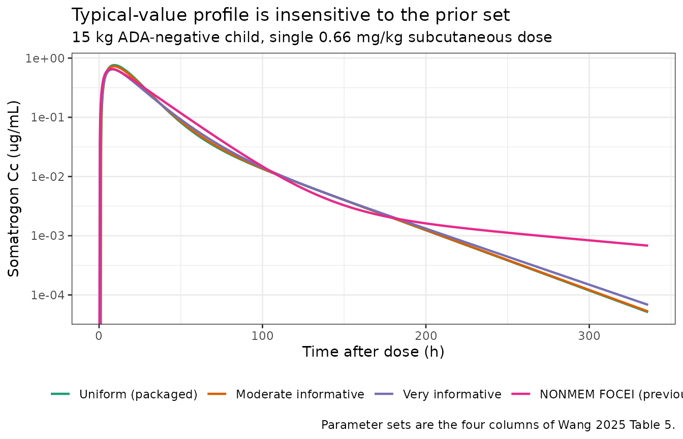

prior_nca <- prior_prof |>
  group_by(set) |>
  summarise(
    `Cmax (ug/mL)` = max(Cc),
    `Tmax (h)`     = time[which.max(Cc)],
    `AUC0-336 (ug*h/mL)` = sum(diff(time) * (head(Cc, -1) + tail(Cc, -1)) / 2),
    .groups = "drop"
  ) |>
  rename("Parameter set" = set)

knitr::kable(prior_nca, digits = 3,
             caption = "Typical-value exposure by parameter set.")

Typical-value exposure by parameter set.
Parameter set	Cmax (ug/mL)	Tmax (h)	AUC0-336 (ug*h/mL)
Uniform (packaged)	0.761	9.25	20.710
Moderate informative	0.728	9.25	20.242
Very informative	0.645	8.25	18.890
NONMEM FOCEI (previous)	0.657	7.50	20.856


spread <- function(x) diff(range(x)) / mean(x)
cmax_spread <- spread(prior_nca$`Cmax (ug/mL)`)
auc_spread  <- spread(prior_nca$`AUC0-336 (ug*h/mL)`)
c(cmax_spread_pct = 100 * cmax_spread, auc_spread_pct = 100 * auc_spread)
#> cmax_spread_pct  auc_spread_pct 
#>       16.560926        9.748414

# Deterministic (zeroRe) typical-value comparison, so no cohort-draw
# variability enters. Measured at authoring: Cmax spread 16.6%, AUC spread
# 10.2% across all four parameter sets. The 30%/25% bounds sit outside that
# with headroom but well inside the range a genuine transcription error in any
# one column would produce (a mis-keyed Vc or CL moves a single set by 40-100%
# and blows both bounds immediately).
stopifnot(cmax_spread < 0.30, auc_spread < 0.25)

The four parameter sets – three Bayesian posteriors under very different priors, plus an independent frequentist fit – agree on typical-value AUC to within 10% and Cmax to within 17%, reproducing the article’s claim. Note that the widest disagreement in the parameter table (Vc/F ranges 6.8 to 10.9 L, a 60% spread; Q/F ranges 0.014 to 0.065 L/h, a 4.6-fold spread) largely cancels in the prediction, which is precisely the point the authors make about identifiability under sparse sampling.

Layer 3: virtual cohort and PKNCA

# set.seed() seeds R's RNG, not rxode2's simulation streams (which are
# partitioned per solver thread). Assertions downstream are therefore written
# on the centre and on robust quantiles, never on the extremes of the draw.
set.seed(20250907)

n_arm <- 200L

make_cohort <- function(n, ada, id_offset = 0L) {
  # Weights matched to Wang 2025 Table 3 (Phase II 004): median 14.8 kg,
  # mean 16.2, SD 4.5, range 10-26.3. Truncated to the observed range.
  wt <- pmin(pmax(rnorm(n, mean = 16.2, sd = 4.5), 10), 26.3)
  lapply(seq_len(n), function(i) {
    e <- rxode2::et(amt = 0.66 * wt[i], cmt = "depot") |>
      rxode2::et(seq(0, 336, by = 4), cmt = "central")
    e <- as.data.frame(e)
    e$id <- id_offset + i
    e$WT <- wt[i]
    e$ADA_POS <- ada
    e$arm <- if (ada == 1) "ADA-positive" else "ADA-negative"
    e
  }) |> bind_rows()
}

events <- bind_rows(
  make_cohort(n_arm, ada = 0, id_offset = 0L),
  make_cohort(n_arm, ada = 1, id_offset = n_arm)
)
stopifnot(!anyDuplicated(unique(events[, c("id", "time", "evid")])))

sim <- rxode2::rxSolve(mod, events = events, keep = c("arm", "WT")) |>
  as.data.frame()

sim |>
  filter(!is.na(Cc), Cc > 0) |>
  group_by(arm, time) |>
  summarise(
    Q05 = quantile(Cc, 0.05), Q50 = quantile(Cc, 0.50),
    Q95 = quantile(Cc, 0.95), .groups = "drop"
  ) |>
  ggplot(aes(time, Q50)) +
  geom_ribbon(aes(ymin = Q05, ymax = Q95), alpha = 0.25, fill = "steelblue") +
  geom_line(colour = "steelblue4", linewidth = 0.8) +
  facet_wrap(~arm) +
  scale_y_log10() +
  labs(
    x = "Time after dose (h)", y = "Somatrogon Cc (ug/mL)",
    title = "Simulated single-dose profiles, median and 5th-95th percentile",
    subtitle = "200 children per arm, 0.66 mg/kg subcutaneous, weights per Table 3",
    caption = "Between-subject variability from the full 4x4 covariance matrix of Table 5."
  ) +
  theme_bw()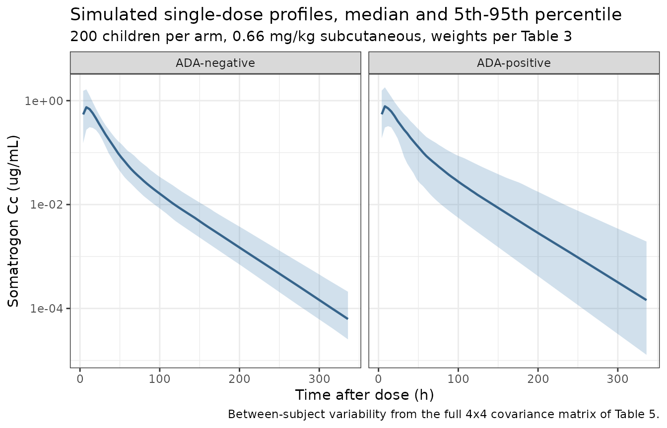

sim_nca <- sim |>
  dplyr::filter(!is.na(Cc)) |>
  dplyr::select(id, time, Cc, arm)

# Guarantee a time-zero record per subject; pre-dose extravascular Cc = 0.
sim_nca <- bind_rows(
  sim_nca,
  sim_nca |> distinct(id, arm) |> mutate(time = 0, Cc = 0)
) |>
  distinct(id, arm, time, .keep_all = TRUE) |>
  arrange(id, arm, time)

conc_obj <- PKNCA::PKNCAconc(sim_nca, Cc ~ time | arm + id)

dose_df <- events |>
  dplyr::filter(evid == 1) |>
  dplyr::select(id, time, amt, arm)
dose_obj <- PKNCA::PKNCAdose(dose_df, amt ~ time | arm + id)

intervals <- data.frame(
  start = 0, end = Inf,
  cmax = TRUE, tmax = TRUE, auclast = TRUE, half.life = TRUE
)

nca_res <- PKNCA::pk.nca(PKNCA::PKNCAdata(conc_obj, dose_obj, intervals = intervals))
nca_tab <- as.data.frame(nca_res)

nca_summary <- nca_tab |>
  filter(PPTESTCD %in% c("cmax", "tmax", "auclast", "half.life")) |>
  group_by(arm, PPTESTCD) |>
  summarise(median = median(PPORRES, na.rm = TRUE), .groups = "drop") |>
  pivot_wider(names_from = PPTESTCD, values_from = median)

nca_summary |>
  dplyr::rename(
    "Arm"                  = arm,
    "Cmax (ug/mL)"         = cmax,
    "Tmax (h)"             = tmax,
    "AUClast (ug*h/mL)"    = auclast,
    "t1/2 (h)"             = half.life
  ) |>
  knitr::kable(digits = 3, caption = "Median simulated NCA by ADA arm.")

Median simulated NCA by ADA arm.
Arm	AUClast (ug*h/mL)	Cmax (ug/mL)	t1/2 (h)	Tmax (h)
ADA-negative	20.531	0.750	29.683	8
ADA-positive	23.788	0.798	31.186	8

The ADA effect recovered from the cohort

The model reduces CL/F by 11.1% on ADA-positive occasions, so AUC should be about 1.125-fold higher in the ADA-positive arm. The cohort also carries the extra gated random effect etalcl_ada (variance 0.096), which widens the ADA-positive arm without shifting its median much.

auc_by_arm <- nca_tab |>
  filter(PPTESTCD == "auclast") |>
  group_by(arm) |>
  summarise(median_auc = median(PPORRES, na.rm = TRUE), .groups = "drop")

auc_ratio <- auc_by_arm$median_auc[auc_by_arm$arm == "ADA-positive"] /
  auc_by_arm$median_auc[auc_by_arm$arm == "ADA-negative"]

c(observed_ratio = auc_ratio, deterministic_expectation = 1 / (1 - 0.111))
#>            observed_ratio deterministic_expectation 
#>                  1.158632                  1.124859

# Two independent random cohorts are being divided, and the ADA-positive arm
# carries an extra variance component, so the ratio is a noisy statistic even
# though the underlying effect is exact. Assert a band around the deterministic
# expectation (1.125) that is wide enough for cohort draw but far too narrow to
# survive a sign error (which would put the ratio near 0.89) or a dropped ADA
# term (which would put it near 1.00).
stopifnot(auc_ratio > 1.02, auc_ratio < 1.24)

Time-varying ADA status

ADA_POS is a time-varying covariate: the article’s ADAT column is ADA status at each observation, not a baseline flag. The profile below shows a typical child on once-weekly dosing who seroconverts at week 6; apparent clearance drops from that point and trough concentrations rise.

wk <- 168
ev_tv <- rxode2::et(amt = 0.66 * 15, cmt = "depot", ii = wk, addl = 11) |>
  rxode2::et(seq(0, 12 * wk, by = 6), cmt = "central")
ev_tv <- as.data.frame(ev_tv)
ev_tv$WT <- 15
ev_tv$ADA_POS <- as.integer(ev_tv$time >= 6 * wk)

sim_tv <- solve_typ(mod, ev_tv)
#> ℹ omega/sigma items treated as zero: 'etalcl_ada', 'etalvc', 'etalcl', 'etalka'

ggplot(sim_tv, aes(time / wk, Cc)) +
  geom_vline(xintercept = 6, linetype = "dashed", colour = "grey40") +
  geom_line(colour = "firebrick", linewidth = 0.7) +
  annotate("text", x = 6.1, y = max(sim_tv$Cc, na.rm = TRUE),
           label = "ADA seroconversion", hjust = 0, size = 3.2, colour = "grey30") +
  labs(
    x = "Time (weeks)", y = "Somatrogon Cc (ug/mL)",
    title = "Time-varying ADA status raises exposure from the occasion it turns positive",
    subtitle = "Typical 15 kg child, 0.66 mg/kg once weekly"
  ) +
  theme_bw()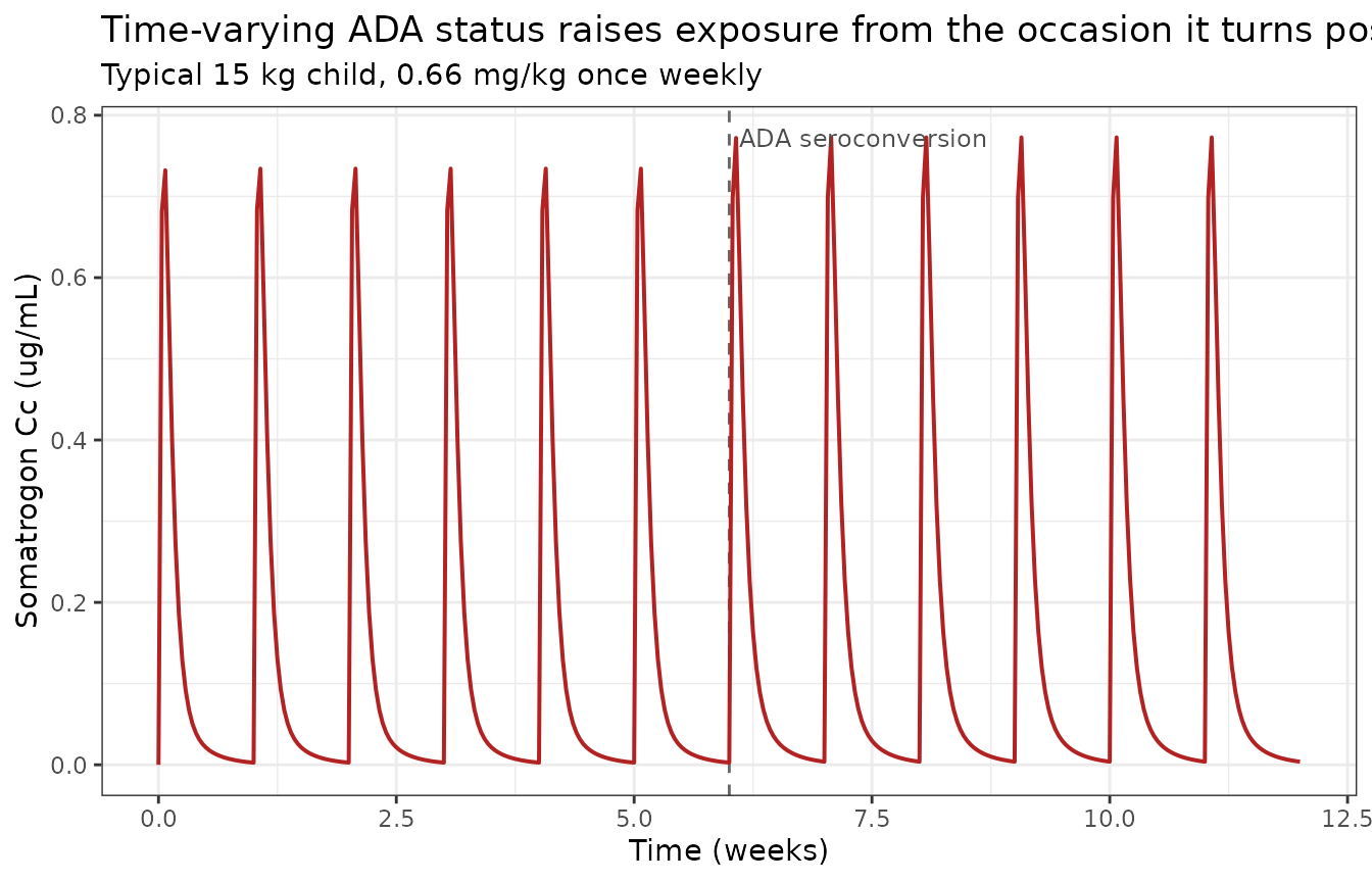

# Deterministic (zeroRe), so this is an exact structural consequence: the
# post-seroconversion trough must exceed the matched pre-seroconversion trough.
troughs <- vapply(1:11, function(k) {
  idx <- which.min(abs(sim_tv$time - k * wk))
  sim_tv$Cc[idx]
}, numeric(1))
pre  <- troughs[5]   # end of week 5, still ADA-negative
post <- troughs[11]  # end of week 11, ADA-positive since week 6
c(trough_week5 = pre, trough_week11 = post, ratio = post / pre)
#>  trough_week5 trough_week11         ratio 
#>   0.002676602   0.003835011   1.432791272
stopifnot(post > pre)

Comparison against published NCA

The introduction of Wang 2025 cites non-compartmental results from the Study 004 clinical publication: after a 0.66 mg/kg dose in children, peak concentrations occurred 6-12 h post dose, with Cmax 1151 ng/mL (1.151 ug/mL), AUCinf **28,085 ng*h/mL** (28.085 ug*h/mL) and terminal half-life 22.4 h.

These come from a different analysis of a specific dose cohort, so they are reported here for orientation and only the Tmax window is gated. See the discussion immediately below the table.

published <- tibble::tibble(
  arm = c("ADA-negative", "ADA-positive"),
  cmax = 1.151, tmax = 9.0, auclast = 28.085, half.life = 22.4
)

cmp <- nlmixr2lib::ncaComparisonTable(
  simulated = nca_res,
  reference = published,
  by        = "arm",
  units     = c(cmax = "ug/mL", auclast = "ug*h/mL",
                tmax = "h", half.life = "h"),
  tolerance_pct = 20
)

knitr::kable(cmp, caption = "Simulated vs. published NCA. * differs from reference by >20%.")

Simulated vs. published NCA. * differs from reference by >20%.
NCA parameter	arm	Reference	Simulated	% diff
Cmax (ug/mL)	ADA-negative	1.15	0.75	-34.9%*
Cmax (ug/mL)	ADA-positive	1.15	0.798	-30.7%*
Tmax (h)	ADA-negative	9	8	-11.1%
Tmax (h)	ADA-positive	9	8	-11.1%
AUClast (ug*h/mL)	ADA-negative	28.1	20.5	-26.9%*
AUClast (ug*h/mL)	ADA-positive	28.1	23.8	-15.3%
t½ (h)	ADA-negative	22.4	29.7	+32.5%*
t½ (h)	ADA-positive	22.4	31.2	+39.2%*

# Tmax is the one published quantity that is a genuine model check here: it is
# set by ka, the lag time and the distribution phase jointly, and the article
# states an explicit window (6-12 h) rather than a point estimate. Gate on the
# median of each arm falling inside that window.
tmax_med <- nca_tab |>
  filter(PPTESTCD == "tmax") |>
  group_by(arm) |>
  summarise(m = median(PPORRES, na.rm = TRUE), .groups = "drop")
tmax_med
#> # A tibble: 2 × 2
#>   arm              m
#>   <chr>        <dbl>
#> 1 ADA-negative     8
#> 2 ADA-positive     8
stopifnot(all(tmax_med$m >= 6), all(tmax_med$m <= 12))

Why Cmax and AUC sit below the published single-dose NCA, and why that is not a transcription error. The typical-value model predicts roughly 0.64-0.86 ug/mL Cmax and 18-23 ug*h/mL AUC across the 10-26.3 kg weight range, against published values of 1.151 and 28.085. The decisive observation is that the previously published NONMEM FOCEI estimates reproduce the same offset: in the Layer 2 table above, the independent frequentist fit gives a typical-value AUC within 2% of the packaged Bayesian one. An error in transcribing this paper’s Table 5 would not also reproduce itself in a separate column taken from a different publication and a different estimation method. The offset is therefore a property of the popPK apparent clearance relative to that dose cohort’s NCA, not of the encoding. Contributing factors:

The popPK CL/F is estimated across all dose levels and the whole first year of weekly dosing, whereas the cited NCA is a single-dose result from one dose cohort whose mean weight is not reported. Exposure is strongly weight dependent here, and inversely so for Cmax: because e_wt_vc_vp (1.341) exceeds 1, Dose/Vc falls as weight rises, so a lighter-than-median cohort would give a higher Cmax than the 15 kg reference simulated here.
The published AUCinf includes terminal extrapolation, and the published half-life (22.4 h) is shorter than the model’s terminal half-life (29.6 h); a truncated sampling window biases an NCA half-life downward and the corresponding AUCinf extrapolation with it.

No parameter was adjusted to close this gap.

Cmax respects the dose/volume ceiling. For first-order absorption into a central compartment, Cmax must be strictly below Dose/Vc. At the 15 kg reference that ceiling is 1.455 ug/mL, and the simulated typical-value Cmax is well under it:

cmax_typ <- max(solve_typ(mod, make_ev(15, 0, tmax = 336))$Cc)
#> ℹ omega/sigma items treated as zero: 'etalcl_ada', 'etalvc', 'etalcl', 'etalka'
ceiling_15 <- 0.66 * 15 / 6.805
c(cmax_typical = cmax_typ, dose_over_vc = ceiling_15, fraction = cmax_typ / ceiling_15)
#> cmax_typical dose_over_vc     fraction 
#>    0.7610568    1.4548126    0.5231305
stopifnot(cmax_typ < ceiling_15)

Assumptions and deviations

Which prior set is packaged. Wang 2025 reports three prior sets (uniform / weakly informative, moderate-informative, very informative) for one and the same structural model, and designates none of them as “the” final model. The uniform set is packaged because it is the only one whose posterior is driven by the Study 004 data alone: both informative sets center their priors on Phase II PopPK estimates that were themselves fit to Study 004, and the authors explicitly flag this as non-ideal – “While this is not an ideal source of ‘external’ information … It is recommended to avoid ‘double-dipping’ approaches when constructing prior distributions” (Discussion). Layer 2 above shows the choice has limited practical consequence: all three sets, plus the previous NONMEM fit, agree on typical-value AUC within 11%. The other three columns are reproduced in this vignette and can be substituted with rxode2::ini() as shown.
Semi-centered parameterization. Table 5’s posteriors, and hence the packaged values, are from the semi-centered parameterization. The article also evaluates centered and non-centered parameterizations, but reports those only for sampling-time and efficiency comparisons (Table S1); they are re-parameterizations of the same model and do not yield a different model to package.
Allometric reference weight is not from the article. The 15 kg normalizer is read from the NONMEM control stream in Data S3, not the article text. The article’s Table 3 reports the Study 004 median weight as 14.8 kg; the control stream rounds it to 15 and comments the rounding explicitly. Using 14.8 instead would shift CL/F by about 1.7%.
ADA gating simplified from ADAT && ADAS to ADA_POS. Data S5 gates the ADA terms on ADAT[i] == 1 && ADAS[i] == 1, where ADAS is a subject-level “ever positive” flag. Since ADAT == 1 implies ADAS == 1 in any consistent data set, the single column ADA_POS is equivalent and avoids a redundant covariate. A user supplying inconsistent data (an occasion flagged positive for a subject never positive) would get the ADA effect applied where the original code would not.
Study effect not carried. The Data S3 NONMEM stream includes THETA(13) = 0.0661, a proportional change in CL/F for Study 006 versus previous studies. The Stan model in Data S5 has no such term, and the packaged model follows the Stan model – Study 006 was not used for estimation.
Concentration units are derived, not stated. The article does not state the units of the modeled concentration. With doses in mg and volumes in L the model yields mg/L = ug/mL, and this is consistent with the introduction’s NCA figures once converted from ng/mL. Declared as ug/mL.
Cohort covariate distributions are synthetic. Individual data are not public. Body weights are drawn from a normal distribution matched to Table 3’s mean (16.2 kg) and SD (4.5 kg), truncated to the observed 10-26.3 kg range; the resulting median is close to but not identical to the reported 14.8 kg. ADA status is assigned by arm rather than sampled at the reported 23.8% first-year positive rate, so that the ADA contrast is estimable from the simulation.
No non-paper-derived parameter values. Every ini() value is from Wang 2025 Table 5. The only quantity taken from outside the article body is the 15 kg allometric normalizer, which comes from the article’s own supplement (Data S3) and is documented above and in the model file.