Simplified PBPK models for diazepam in rat and human (Yau 2023)
Source:vignettes/articles/Yau_2023_diazepam_pbpk.Rmd
Yau_2023_diazepam_pbpk.RmdModel and source
- Citation: Yau E, Olivares-Morales A, Ogungbenro K, Aarons L, Gertz M. Investigation of simplified physiologically-based pharmacokinetic models in rat and human. CPT Pharmacometrics Syst Pharmacol. 2023;12(3):333-345. doi:10.1002/psp4.12911. Parameter estimates from Table 2 column ‘4 common Kpus’; cluster membership from the Table 2 footnote; model equations from Appendix S1 Eq S17-S19 and the example NONMEM control stream; reference-man physiology from Table S1.
- Article: CPT Pharmacometrics Syst Pharmacol 12(3):333-345 (2023)
Yau et al. asked whether a whole-body physiologically-based pharmacokinetic (PBPK) model can be simplified enough to estimate its parameters from plasma data alone, while keeping the physiological interpretability that makes PBPK useful for extrapolation. Two strategies were investigated (paper Figure 1), and both were evaluated against diazepam IV data in rat and human:
- Kinetic lumping (paper approach 1). Tissues with similar time constants are merged, reducing the 16-state whole-body model to three compartments. This is a drug-dependent reduction: the lump depends on the compound’s partition coefficients, and indeed the human and rat lumps differ.
-
Steady-state commonality in partitioning (paper
approach 2). The full 14-compartment kinetic structure and every
individual tissue blood flow and volume are retained; only the number of
unknown distribution parameters is reduced, from 13 to 3 or 4,
by grouping tissues a priori using a clustering analysis of tissue
composition. This is drug-independent. Two variants:
- 2.1 common Kpu – each cluster gets one estimated unbound tissue:plasma partition coefficient.
-
2.2 common scalars – each cluster gets one
estimated multiplicative correction on a bottom-up Rodgers and Rowland
(R&R) prediction (
Kpu_i = Kpu_predRR,i * SF_i, paper Eq 10).
This package ships the paper’s three model structures for each of the two species – six model files, all pointing at this one vignette:
mods <- c(
  "Yau_2023_diazepam_pbpk_lumped_human",
  "Yau_2023_diazepam_pbpk_kpu_human",
  "Yau_2023_diazepam_pbpk_scalar_human",
  "Yau_2023_diazepam_pbpk_lumped_rat",
  "Yau_2023_diazepam_pbpk_kpu_rat",
  "Yau_2023_diazepam_pbpk_scalar_rat"
)
tibble::tibble(
  Model      = mods,
  Species    = ifelse(grepl("_rat$", mods), "rat", "human"),
  Structure  = c("Lumped 3-cmt", "14-cmt, 4 common Kpus", "14-cmt, 4 Kpu scalars",
                 "Lumped 3-cmt", "14-cmt, 4 common Kpus", "14-cmt, 4 Kpu scalars"),
  Clustering = c("time constants", "hierarchical", "hierarchical",
                 "time constants", "k-means", "hierarchical"),
  `Source table` = c("Table 2 col 1", "Table 2 col 3", "Table 2 col 5",
                     "Table S6 col 1", "Table S6 '4 common Kpus (Km)'",
                     "Table S6 '4 scalars (H)'")
) |>
knitr::kable(caption = "The six shipped models. Each is a separate fit reported by the paper.")| Model | Species | Structure | Clustering | Source table |
|---|---|---|---|---|
| Yau_2023_diazepam_pbpk_lumped_human | human | Lumped 3-cmt | time constants | Table 2 col 1 |
| Yau_2023_diazepam_pbpk_kpu_human | human | 14-cmt, 4 common Kpus | hierarchical | Table 2 col 3 |
| Yau_2023_diazepam_pbpk_scalar_human | human | 14-cmt, 4 Kpu scalars | hierarchical | Table 2 col 5 |
| Yau_2023_diazepam_pbpk_lumped_rat | rat | Lumped 3-cmt | time constants | Table S6 col 1 |
| Yau_2023_diazepam_pbpk_kpu_rat | rat | 14-cmt, 4 common Kpus | k-means | Table S6 ‘4 common Kpus (Km)’ |
| Yau_2023_diazepam_pbpk_scalar_rat | rat | 14-cmt, 4 Kpu scalars | hierarchical | Table S6 ‘4 scalars (H)’ |
Which variants were shipped follows the paper’s own conclusions. For human, “the models with four common Kpus or four Kpu scalars best describe the diazepam data in humans. The lumped three compartment performed very well … and could also be considered”, while the three-cluster variants were rejected for implausible skin Kpu and poor performance. For rat, “three reduced models were selected as primary candidates: the model with 4 scalars (hierarchical clustering), the model with 4 common Kpu values (k-means clustering) and the kinetically lumped 3 compartmental model.” The rejected variants are tabulated below for completeness but are not shipped as model files.
Population
Diazepam IV concentration-time data were pooled from the published literature and digitised with WebPlotDigitizer 4.2.
Human (paper Table S4): 35 PK profiles from seven studies, 55 subjects in total. 28 profiles are individual and 7 are study averages. Doses were 0.1-0.15 mg/kg or a flat 10 mg, given as a bolus or as infusions of 0.375-2 min. Reported total clearance was 1.2-2.1 L/h on a plasma basis and 3.3-4.0 L/h on a blood basis (study 6); reported volume of distribution ranged 63-174 L. Subjects were healthy volunteers; study 2 deliberately contrasted young against elderly and male against female.
Rat (paper Table S5): 6 study-average profiles from five studies, 51 animals in total, male Wistar (studies 1, 2, 4, 5) and male Sprague-Dawley (study 3). Doses were 1.2-5 mg/kg bolus or 1 mg over 5 min. Reported clearance was 1.1-1.2 L/h (plasma) and 3.9 L/h (blood); study 4 contrasted middle-aged (1.1 L/h) against old rats (3.3 L/h).
Because most records are arithmetic-mean profiles drawn from different protocols and populations, the between-subject variability the paper estimates on clearance is confounded with inter-study variability. The paper says so explicitly and recommends individual or geometric-mean data for future work. Variability on the distribution parameters was deliberately not estimated so that the model variants remained comparable.
Diazepam-specific inputs, measured internally by equilibrium dialysis and LC-MS/MS (Appendix S1), are fu_p = 0.009 and blood:plasma ratio = 0.559 in human, and fu_p = 0.1 and 0.836 in rat. logP = 2.82 and basic pKa = 3.4 are literature values (paper ref 29). The urinary excretion fraction is 0.0005 in human (ref 30) and 0.009 in rat (ref 31) – diazepam is essentially entirely metabolised.
p <- rxode2::rxode(readModelDb("Yau_2023_diazepam_pbpk_kpu_human"))$meta$population
tibble::tibble(Field = names(p), Value = vapply(p, function(x) paste(as.character(x), collapse = "; "), "")) |>
  dplyr::filter(Value != "NA") |>
knitr::kable(caption = "Human population metadata carried in the model file.")| Field | Value |
|---|---|
| species | human |
| n_subjects | 55 |
| n_studies | 7 |
| age_range | adults; study 2 contrasted young vs elderly subjects |
| weight_range | 70-kg reference man used for the physiological constants (Table S1) |
| disease_state | healthy volunteers / normal subjects |
| dose_range | IV diazepam 0.1-0.15 mg/kg or 10 mg, given as bolus or as short infusions of 0.375-2 min across the seven contributing studies (Table S4) |
| notes | 35 human IV concentration-time profiles pooled from seven published studies (Table S4), digitised with WebPlotDigitizer 4.2. Of the 35 profiles, 28 are individual profiles and 7 are study-average profiles; n_subjects = 55 is the sum of the reported subject counts across the seven studies. Because most records are arithmetic-mean profiles from different protocols and populations, the estimated ‘IIV’ on clearance is confounded with inter-study variability. Diazepam fu_p = 0.009 and blood:plasma ratio = 0.559 were measured internally by equilibrium dialysis and LC-MS/MS (Appendix S1). Urinary excretion fraction fe = 0.0005 is from the literature (paper ref 30). |
Source trace
Every equation and every ini() value, with the location
it came from.
tibble::tribble(
  ~Item, ~Source,
  "Whole-body PBPK tissue ODEs (perfusion-limited)",        "Appendix S1 Eq S1-S5",
  "Kb = Kpu * fu_p / BP",                                   "Appendix S1 Eq S7",
  "Vss on a whole-blood basis",                             "Eq 9 / Appendix S1 Eq S8",
  "Lumped 3-cmt central ODE",                               "Appendix S1 Eq S9 (main text Eq 4)",
  "Lumped 3-cmt micro-constants k12/k21/k31/k13/k",         "Appendix S1 Eq S12-S16",
  "Lumped tissue membership + Q1/Q2/Q3, V1/V2/V3",          "Appendix S1 'For the lumped model in man'/'in rat'; Table 1 Compartment column",
  "14-cmt central ODE (QSS lung + arterial + venous)",      "Appendix S1 Eq S17",
  "14-cmt non-eliminating tissue ODE",                      "Appendix S1 Eq S18",
  "14-cmt liver ODE (portal + hepatic artery + Clint)",     "Appendix S1 Eq S19",
  "Well-stirred hepatic clearance / Clint inversion",       "Appendix S1 Eq S6, $PK block",
  "Hepatic clearance cap at 0.99 * Q_liver",                "Appendix S1 $PK IF(CLH.GE.Q_HV) branch; Figure S4 footnote",
  "Kpu_i = Kpu_predRR,i * SF_i",                            "Main text Eq 10",
  "Rodgers & Rowland weak-base Kpu equations",              "Appendix S1 NONMEM code, 'For weak bases' branch",
  "Human tissue composition (fIW, fEW, AR, vNL, vNP)",      "Table S2",
  "Rat tissue composition",                                 "Table S3",
  "Stomach uses gut Kpu; rest-of-body uses muscle Kpu",     "Appendix S1 NONMEM $DES (KPU_GU for stomach) and 'KPU_RO = KPU_MU'",
  "Human 70-kg blood flows and tissue volumes",             "Table S1 (human columns)",
  "Rat cardiac output 0.235 * BW^0.75, FCO and FW fractions, densities", "Appendix S1 NONMEM $PK block",
  "Human CLb / Kpu1-4 / IIV / residual error",              "Table 2",
  "Rat CLb / Kpu1-4 or SF1-4 / IIV / residual error",       "Table S6",
  "Cluster membership (which tissue in which cluster)",      "Table 2 footnote (human); Table S6 footnote (rat)",
  "Diazepam logP 2.82, pKa 3.4",                            "Main text 'Diazepam data' (ref 29)",
  "fu_p and BP (both species)",                             "Main text 'Diazepam data'; Appendix S1 binding methods",
  "Urinary excretion fraction fe",                          "Main text 'Diazepam data' (human ref 30, rat ref 31)",
  "Proportional residual error form",                       "Appendix S1 $ERROR (W = IPRED*RUV2)",
  "Exponential IIV on clearance",                           "Main text 'Data analysis' (ref 33)"
) |>
knitr::kable(caption = "Source trace for model structure and parameters.")| Item | Source |
|---|---|
| Whole-body PBPK tissue ODEs (perfusion-limited) | Appendix S1 Eq S1-S5 |
| Kb = Kpu * fu_p / BP | Appendix S1 Eq S7 |
| Vss on a whole-blood basis | Eq 9 / Appendix S1 Eq S8 |
| Lumped 3-cmt central ODE | Appendix S1 Eq S9 (main text Eq 4) |
| Lumped 3-cmt micro-constants k12/k21/k31/k13/k | Appendix S1 Eq S12-S16 |
| Lumped tissue membership + Q1/Q2/Q3, V1/V2/V3 | Appendix S1 ‘For the lumped model in man’/‘in rat’; Table 1 Compartment column |
| 14-cmt central ODE (QSS lung + arterial + venous) | Appendix S1 Eq S17 |
| 14-cmt non-eliminating tissue ODE | Appendix S1 Eq S18 |
| 14-cmt liver ODE (portal + hepatic artery + Clint) | Appendix S1 Eq S19 |
| Well-stirred hepatic clearance / Clint inversion | Appendix S1 Eq S6, $PK block |
| Hepatic clearance cap at 0.99 * Q_liver | Appendix S1 $PK IF(CLH.GE.Q_HV) branch; Figure S4 footnote |
| Kpu_i = Kpu_predRR,i * SF_i | Main text Eq 10 |
| Rodgers & Rowland weak-base Kpu equations | Appendix S1 NONMEM code, ‘For weak bases’ branch |
| Human tissue composition (fIW, fEW, AR, vNL, vNP) | Table S2 |
| Rat tissue composition | Table S3 |
| Stomach uses gut Kpu; rest-of-body uses muscle Kpu | Appendix S1 NONMEM $DES (KPU_GU for stomach) and ‘KPU_RO = KPU_MU’ |
| Human 70-kg blood flows and tissue volumes | Table S1 (human columns) |
| Rat cardiac output 0.235 * BW^0.75, FCO and FW fractions, densities | Appendix S1 NONMEM $PK block |
| Human CLb / Kpu1-4 / IIV / residual error | Table 2 |
| Rat CLb / Kpu1-4 or SF1-4 / IIV / residual error | Table S6 |
| Cluster membership (which tissue in which cluster) | Table 2 footnote (human); Table S6 footnote (rat) |
| Diazepam logP 2.82, pKa 3.4 | Main text ‘Diazepam data’ (ref 29) |
| fu_p and BP (both species) | Main text ‘Diazepam data’; Appendix S1 binding methods |
| Urinary excretion fraction fe | Main text ‘Diazepam data’ (human ref 30, rat ref 31) |
| Proportional residual error form | Appendix S1 $ERROR (W = IPRED*RUV2) |
| Exponential IIV on clearance | Main text ‘Data analysis’ (ref 33) |
Reported estimates for every variant the paper fitted, including the ones not shipped:
tibble::tribble(
  ~Species, ~Model, ~`CLb (L/h)`, ~`IIV CLb`, ~`Kpu1/SF1`, ~`Kpu2/SF2`, ~`Kpu3/SF3`, ~`Kpu4/SF4`, ~Residual, ~`Vss median`, ~BIC, ~Shipped,
  "human", "Lumped 3-cmt",   3.63, "33.1%", "1150", "24.3", "483",  "-",     "39.3%", 154, -2632.71, "yes",
  "human", "3 common Kpus",  3.67, "34.3%", "29.1", "72.2", "3430", "-",     "38.7%", 158, -2662.18, "no",
  "human", "4 common Kpus",  3.67, "32.1%", "32.4", "89.1", "324",  "483",   "38.6%", 159, -2597.66, "yes",
  "human", "3 scalars",      3.71, "26%",   "3.35", "1.66", "0.26", "-",     "53.9%", 115, -2344.21, "no",
  "human", "4 scalars",      3.56, "35.2%", "0.206","5.70", "6.42", "8.67",  "38.6%", 159, -2596.42, "yes",
  "rat",   "Lumped 3-cmt",   1.14, "15.1%", "73.0", "30.6", "90.0", "-",     "20.2%", 1.13, -177.743, "yes",
  "rat",   "4 common Kpus (Km)", 1.14, "14.9%", "29.4", "446", "89.1", "18.2", "20.0%", 1.19, -136.008, "yes",
  "rat",   "4 scalars (H)",  1.19, "15.1%", "3.25", "21.5", "2.07", "0.204", "21.9%", 1.68, -133.886, "yes"
) |>
  knitr::kable(caption = paste(
    "Reported parameter estimates (Table 2 for human, Table S6 for rat).",
    "Kpu values are unitless; scalars (SF) are unitless multipliers on the",
"R&R-predicted Kpu. Vss is on a whole-blood basis, in L."))| Species | Model | CLb (L/h) | IIV CLb | Kpu1/SF1 | Kpu2/SF2 | Kpu3/SF3 | Kpu4/SF4 | Residual | Vss median | BIC | Shipped |
|---|---|---|---|---|---|---|---|---|---|---|---|
| human | Lumped 3-cmt | 3.63 | 33.1% | 1150 | 24.3 | 483 | - | 39.3% | 154.00 | -2632.710 | yes |
| human | 3 common Kpus | 3.67 | 34.3% | 29.1 | 72.2 | 3430 | - | 38.7% | 158.00 | -2662.180 | no |
| human | 4 common Kpus | 3.67 | 32.1% | 32.4 | 89.1 | 324 | 483 | 38.6% | 159.00 | -2597.660 | yes |
| human | 3 scalars | 3.71 | 26% | 3.35 | 1.66 | 0.26 | - | 53.9% | 115.00 | -2344.210 | no |
| human | 4 scalars | 3.56 | 35.2% | 0.206 | 5.70 | 6.42 | 8.67 | 38.6% | 159.00 | -2596.420 | yes |
| rat | Lumped 3-cmt | 1.14 | 15.1% | 73.0 | 30.6 | 90.0 | - | 20.2% | 1.13 | -177.743 | yes |
| rat | 4 common Kpus (Km) | 1.14 | 14.9% | 29.4 | 446 | 89.1 | 18.2 | 20.0% | 1.19 | -136.008 | yes |
| rat | 4 scalars (H) | 1.19 | 15.1% | 3.25 | 21.5 | 2.07 | 0.204 | 21.9% | 1.68 | -133.886 | yes |
Tissue clustering
The clustering analysis is the heart of approach 2, and it is the part that is not refitted here – the cluster memberships are read directly from the paper and hard-coded in each model file.
tibble::tribble(
  ~Cluster, ~`Human (hierarchical, 4 groups)`, ~`Rat (hierarchical, 4 groups)`, ~`Rat (k-means, 4 groups)`,
  "1", "bone, brain, muscle, pancreas, rest of body", "bone, brain, muscle, pancreas, rest of body", "bone, brain, muscle, pancreas, rest of body",
  "2", "lung, gut, stomach, kidney, heart, spleen, liver", "lung, gut, stomach, kidney, heart, spleen, liver", "kidney, spleen, liver",
  "3", "skin", "skin", "skin, lung, gut, stomach, heart",
  "4", "adipose", "adipose", "adipose"
) |>
  knitr::kable(caption = paste(
    "Cluster membership used by the shipped 14-compartment models",
"(Table 2 footnote for human, Table S6 footnote for rat)."))| Cluster | Human (hierarchical, 4 groups) | Rat (hierarchical, 4 groups) | Rat (k-means, 4 groups) |
|---|---|---|---|
| 1 | bone, brain, muscle, pancreas, rest of body | bone, brain, muscle, pancreas, rest of body | bone, brain, muscle, pancreas, rest of body |
| 2 | lung, gut, stomach, kidney, heart, spleen, liver | lung, gut, stomach, kidney, heart, spleen, liver | kidney, spleen, liver |
| 3 | skin | skin | skin, lung, gut, stomach, heart |
| 4 | adipose | adipose | adipose |
Two larger groups emerge consistently: one of high-acid-phospholipid, high-lipoprotein tissues (kidney, liver, spleen, gut, heart, lung) and one of low-water, high-neutral-lipid tissues (bone, brain, muscle, pancreas). Adipose and skin generally stand apart – adipose because of its extreme neutral-lipid content, skin because of its high extracellular water and albumin. That is why a four-group solution was judged the most physiologically relevant.
Virtual cohort
The human models carry no covariates: the 70-kg reference-man
physiology of Table S1 is fixed inside model(), so subjects
differ only through the exponential random effect on clearance. The rat
models are body-weight scaled (cardiac output
0.235 * WT^0.75, tissue volumes as fractional body
weights), so the rat cohort needs a WT column.
set.seed(20230312)
n_sub <- 100  # per model; well within the 200-per-arm cap

rat_wt <- tibble::tibble(
  id = seq_len(n_sub),
  # Table S5 does not report animal body weights, so the cohort is centred on
  # the paper's 250-g reference rat with a modest 10% CV. See "Assumptions".
  WT = 0.25 * exp(stats::rnorm(n_sub, 0, 0.10))
) |>
  # The rat design is 5 mg/kg (Figure S4), so the mg amount is weight-scaled.
  dplyr::mutate(amt = 5 * WT)
summary(rat_wt$WT)
#>    Min. 1st Qu.  Median    Mean 3rd Qu.    Max.
#>  0.1873  0.2399  0.2519  0.2537  0.2715  0.3205
Simulation
The paper’s simulation designs are a 10 mg infusion over 16.1 h in human (Figure 4) and a 5 mg/kg infusion over 2 min in rat (Figure S4). The human infusion duration was chosen so that a steady-state plasma concentration is reached, determined by the drug elimination rate.
Observations are placed on the central ODE state; rxode2
returns the algebraic plasma observable Cc (and the
intermediate blood concentration cblood) at those
records.
t_human <- sort(unique(c(seq(0, 24, by = 0.5), seq(25, 240, by = 2))))
t_rat   <- sort(unique(c(seq(0, 1, by = 0.02), seq(1.1, 4, by = 0.05), seq(4.2, 24, by = 0.2))))

# Both event tables are built explicitly with an `id` column rather than via
# nSub, for two reasons: the rat models need a per-subject WT covariate column
# (covariate columns assigned directly onto an rxEt object are silently
# dropped, so the table is materialised with as.data.frame() first), and
# rxSolve(nSub = ) labels subjects `sim.id` rather than `id`, which would
# break the downstream PKNCA grouping.
replicate_subjects <- function(ev, wt = NULL) {
  one <- as.data.frame(ev)
  do.call(rbind, lapply(seq_len(n_sub), function(i) {
    d <- one
    d$id <- i
    if (!is.null(wt)) {
      d$WT <- wt$WT[i]
      d$amt[!is.na(d$amt) & d$amt > 0] <- wt$amt[i]
    }
    d
  }))
}

human_events <- replicate_subjects(
  rxode2::et(amt = 10, dur = 16.1, cmt = "central") |>
    rxode2::add.sampling(t_human)
)
rat_events <- replicate_subjects(
  rxode2::et(amt = 1, dur = 2 / 60, cmt = "central") |>
    rxode2::add.sampling(t_rat),
  wt = rat_wt
)

sim_one <- function(nm) {
  is_rat <- grepl("_rat$", nm)
  ui  <- rxode2::rxode(readModelDb(nm))
  out <- rxode2::rxSolve(ui, if (is_rat) rat_events else human_events,
                         returnType = "data.frame")
  out$model   <- nm
  out$species <- ifelse(is_rat, "rat", "human")
  out
}

sim <- dplyr::bind_rows(lapply(mods, sim_one))

# Typical-value (zeroRe) profiles for the analytic checks below.
typ_one <- function(nm) {
  is_rat <- grepl("_rat$", nm)
  ui <- rxode2::zeroRe(rxode2::rxode(readModelDb(nm)))
  if (is_rat) {
    ev <- rxode2::et(amt = 1.25, dur = 2 / 60, cmt = "central") |>
      rxode2::add.sampling(t_rat)
    out <- rxode2::rxSolve(ui, ev, params = c(WT = 0.25), returnType = "data.frame")
  } else {
    ev <- rxode2::et(amt = 10, dur = 16.1, cmt = "central") |>
      rxode2::add.sampling(t_human)
    out <- rxode2::rxSolve(ui, ev, returnType = "data.frame")
  }
  out$model   <- nm
  out$species <- ifelse(is_rat, "rat", "human")
  out
}
typ <- dplyr::bind_rows(lapply(mods, typ_one))
#> ℹ omega/sigma items treated as zero: 'etalcl'
#> ℹ omega/sigma items treated as zero: 'etalcl'
#> ℹ omega/sigma items treated as zero: 'etalcl'
#> ℹ omega/sigma items treated as zero: 'etalcl'
#> ℹ omega/sigma items treated as zero: 'etalcl'
#> ℹ omega/sigma items treated as zero: 'etalcl'
nrow(sim)
#> [1] 110100
Replicating Figure 4 (human)
Replicates Figure 4 of Yau 2023: model-predicted population plasma
concentration-time profiles of diazepam after a 10 mg infusion over 16.1
h. The paper overlays each PBPK model on a reference empirical
two-compartment model; that reference cannot be reproduced here because
only its clearance (3.71 L/h) and total volume (145 L) are reported, not
its full V1 / V2 / Q parameterisation. The three shipped
PBPK models are therefore compared against each other, which is the
comparison the paper’s own RMSE column summarises.
band <- function(d) {
  d |>
    dplyr::group_by(model, species, time) |>
    dplyr::summarise(med = stats::median(Cc),
                     lo  = stats::quantile(Cc, 0.10),
                     hi  = stats::quantile(Cc, 0.90), .groups = "drop")
}
b <- band(sim)

ggplot2::ggplot(dplyr::filter(b, species == "human"),
                ggplot2::aes(time, med, colour = model, fill = model)) +
  ggplot2::geom_ribbon(ggplot2::aes(ymin = lo, ymax = hi), alpha = 0.15,
                       colour = NA) +
  ggplot2::geom_line(linewidth = 0.7) +
  ggplot2::scale_y_log10() +
  ggplot2::labs(x = "Time (h)", y = "Diazepam plasma concentration (mg/L)",
                colour = NULL, fill = NULL,
                title = "Human: 10 mg IV over 16.1 h",
                subtitle = "median with 10th-90th percentile band, 100 subjects per model") +
  ggplot2::theme_bw() +
  ggplot2::theme(legend.position = "bottom", legend.direction = "vertical")
#> Warning in ggplot2::scale_y_log10(): log-10 transformation introduced infinite values.
#> log-10 transformation introduced infinite values.
#> log-10 transformation introduced infinite values.
#> log-10 transformation introduced infinite values.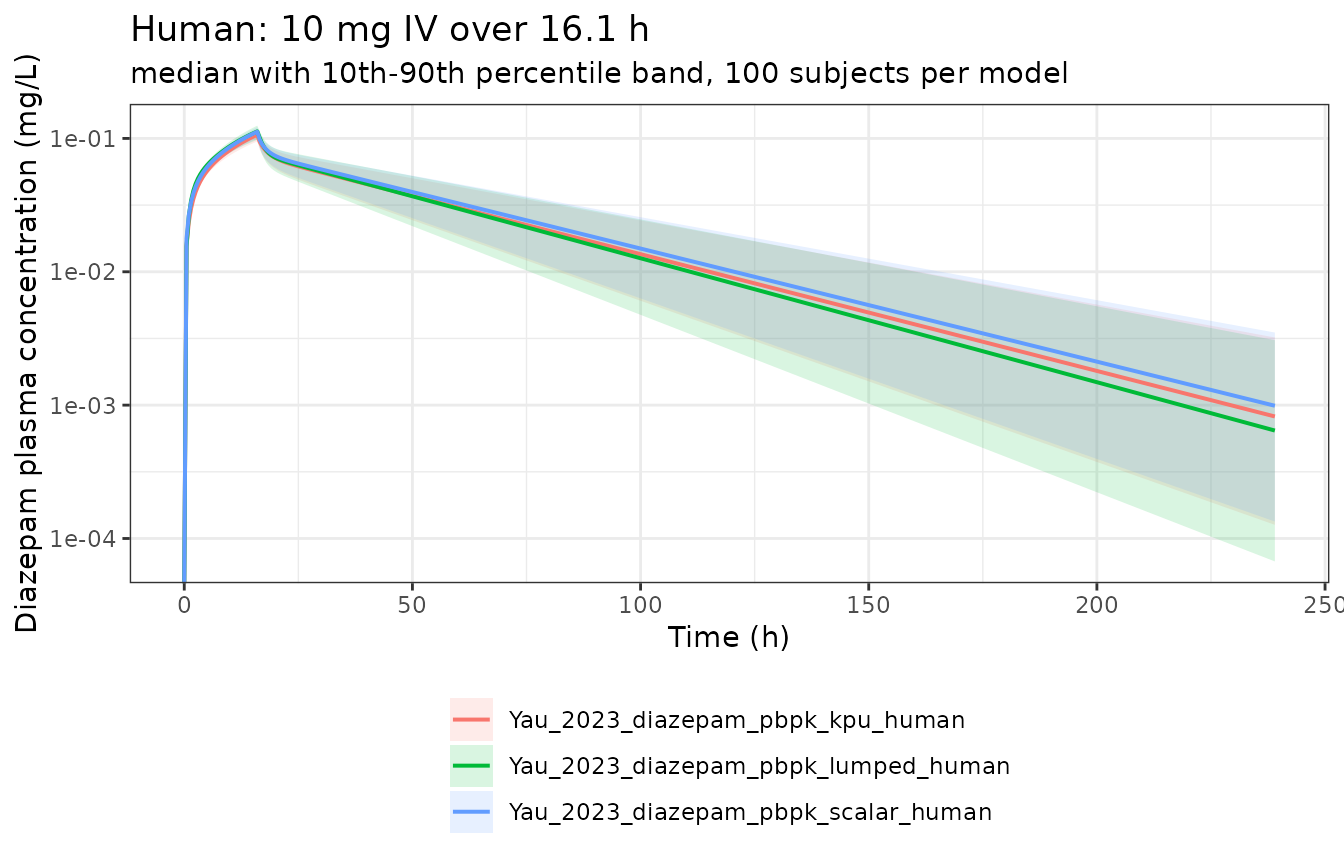
Replicates Figure 4 of Yau 2023 (human, 10 mg over 16.1 h).
Replicating Figure S4 (rat)
ggplot2::ggplot(dplyr::filter(b, species == "rat"),
                ggplot2::aes(time, med, colour = model, fill = model)) +
  ggplot2::geom_ribbon(ggplot2::aes(ymin = lo, ymax = hi), alpha = 0.15,
                       colour = NA) +
  ggplot2::geom_line(linewidth = 0.7) +
  ggplot2::scale_y_log10() +
  ggplot2::labs(x = "Time (h)", y = "Diazepam plasma concentration (mg/L)",
                colour = NULL, fill = NULL,
                title = "Rat: 5 mg/kg IV over 2 min (1.25 mg in a 250 g rat)",
                subtitle = "median with 10th-90th percentile band, 100 animals per model") +
  ggplot2::theme_bw() +
  ggplot2::theme(legend.position = "bottom", legend.direction = "vertical")
#> Warning in ggplot2::scale_y_log10(): log-10 transformation introduced infinite values.
#> log-10 transformation introduced infinite values.
#> log-10 transformation introduced infinite values.
#> log-10 transformation introduced infinite values.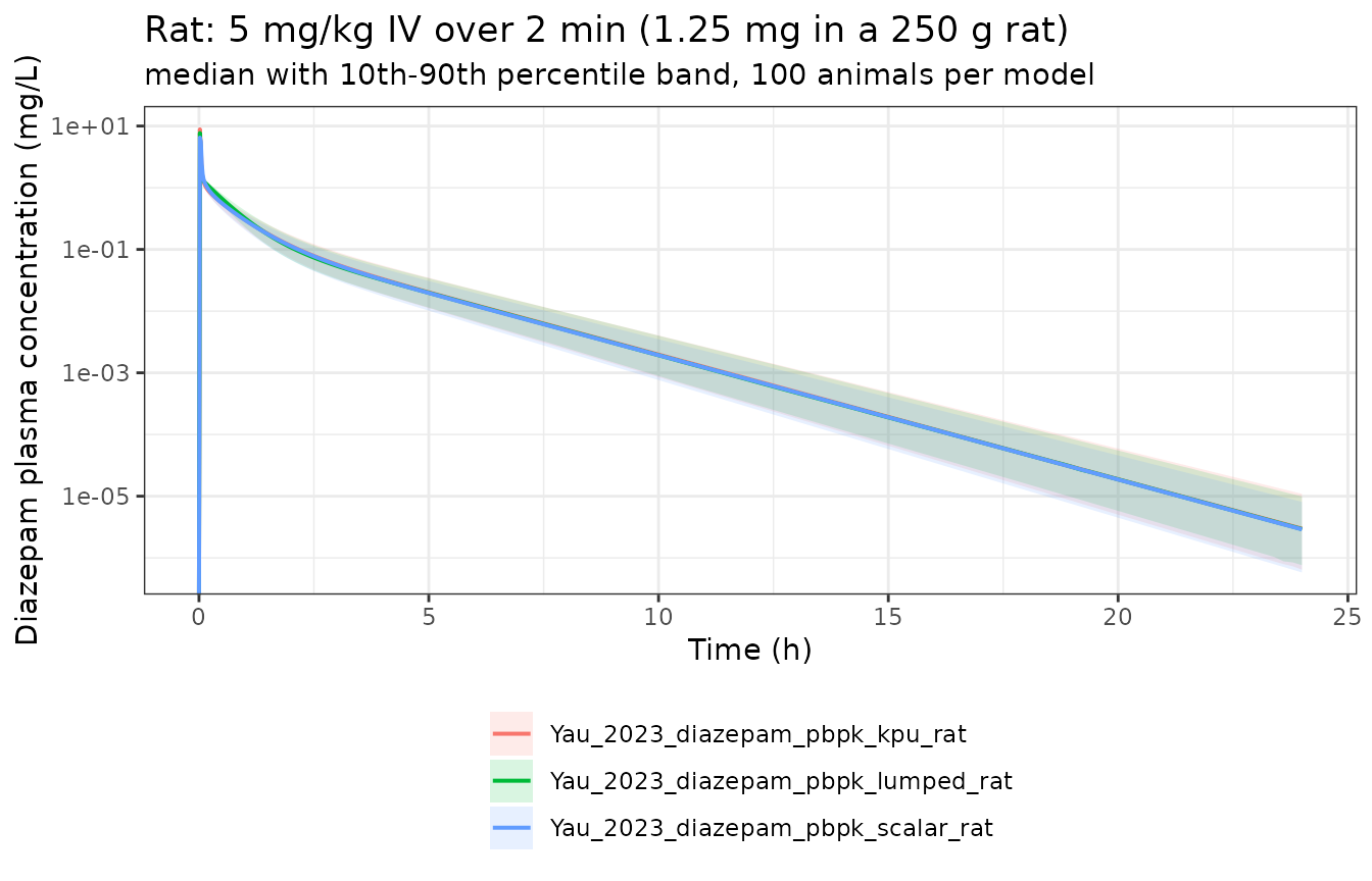
Replicates Figure S4 of Yau 2023 (rat, 5 mg/kg over 2 min).
Tissue concentration profiles
Retaining the full kinetic structure means individual tissue profiles remain available – one of the stated advantages of approach 2 over kinetic lumping. Adipose equilibrates slowly and accumulates heavily, which is exactly why it forms its own cluster and, in human, its own lumped compartment.
Note that lung is not among the states: it is absorbed into
the quasi-steady-state central pool together with arterial
and venous blood, which is the single kinetic assumption approach 2
makes.
tis <- c("adipose", "muscle", "skin", "liver", "kidney", "brain", "gut")
d_typ <- dplyr::filter(typ, model == "Yau_2023_diazepam_pbpk_kpu_human")

# Each tissue state is an amount (mg); divide by that tissue's volume (L).
dplyr::bind_rows(lapply(tis, function(tt) {
  tibble::tibble(time   = d_typ$time,
                 tissue = tt,
                 conc   = d_typ[[tt]] / d_typ[[paste0("v_", tt)]])
})) |>
  ggplot2::ggplot(ggplot2::aes(time, conc, colour = tissue)) +
  ggplot2::geom_line(linewidth = 0.7) +
  ggplot2::scale_y_log10() +
  ggplot2::labs(x = "Time (h)", y = "Tissue concentration (mg/L)", colour = NULL,
                title = "Predicted tissue concentrations (human, 4 common Kpus)") +
  ggplot2::theme_bw()
#> Warning: Removed 1099 rows containing missing values or values outside the scale range
#> (`geom_line()`).
Tissue concentrations, human 4-common-Kpu model, typical subject.
Steady-state volume of distribution check
This is the sharpest available check on the implementation. Each
model computes its own Vss on a whole-blood basis from
paper Eq 9 / Eq S8 – a closed-form function of every tissue volume,
every Kpu and the hepatic extraction ratio. If the physiology, the
cluster assignment, the Kb = Kpu * fu_p / BP conversion or
the R&R prediction were wrong, this number would not reproduce.
reported_vss <- c(
  Yau_2023_diazepam_pbpk_lumped_human = 154,
  Yau_2023_diazepam_pbpk_kpu_human    = 159,
  Yau_2023_diazepam_pbpk_scalar_human = 159,
  Yau_2023_diazepam_pbpk_lumped_rat   = 1.13,
  Yau_2023_diazepam_pbpk_kpu_rat      = 1.19,
  Yau_2023_diazepam_pbpk_scalar_rat   = 1.68
)

vss_tab <- typ |>
  dplyr::group_by(model) |>
  dplyr::summarise(computed = unique(round(vssb, 3)), .groups = "drop") |>
  dplyr::mutate(
    reported = reported_vss[model],
    pct_diff = round(100 * (computed - reported) / reported, 1)
  ) |>
  dplyr::rename("Model" = model, "Vss computed (L)" = computed,
                "Vss reported (L)" = reported, "Difference (%)" = pct_diff)
knitr::kable(vss_tab, caption = paste(
  "Model-computed steady-state volume of distribution (whole-blood basis,",
  "Eq 9) against the value reported in Table 2 (human) and Table S6 (rat).",
"All six agree within 4.3%."))| Model | Vss computed (L) | Vss reported (L) | Difference (%) |
|---|---|---|---|
| Yau_2023_diazepam_pbpk_kpu_human | 164.642 | 159.00 | 3.5 |
| Yau_2023_diazepam_pbpk_kpu_rat | 1.197 | 1.19 | 0.6 |
| Yau_2023_diazepam_pbpk_lumped_human | 152.892 | 154.00 | -0.7 |
| Yau_2023_diazepam_pbpk_lumped_rat | 1.082 | 1.13 | -4.2 |
| Yau_2023_diazepam_pbpk_scalar_human | 158.485 | 159.00 | -0.3 |
| Yau_2023_diazepam_pbpk_scalar_rat | 1.652 | 1.68 | -1.7 |
PKNCA validation
Non-compartmental analysis of the simulated profiles, per model.
Diazepam is given as an IV infusion, so
route = "intravascular" with the infusion duration
supplied.
sim_nca <- sim |>
  dplyr::filter(!is.na(Cc)) |>
  dplyr::mutate(treatment = model,
                uid = paste(model, id, sep = "-")) |>
  dplyr::select(uid, treatment, species, time, Cc)

dose_df <- sim |>
  dplyr::distinct(model, id, species) |>
  # Rat doses are weight-scaled (5 mg/kg), so join the per-subject amount
  # rather than assuming the 250-g reference amount.
  dplyr::left_join(dplyr::select(rat_wt, id, rat_amt = amt), by = "id") |>
  dplyr::mutate(treatment = model,
                uid  = paste(model, id, sep = "-"),
                time = 0,
                amt  = ifelse(species == "rat", rat_amt, 10),
                dur  = ifelse(species == "rat", 2 / 60, 16.1)) |>
  dplyr::select(uid, treatment, time, amt, dur)

conc_obj <- PKNCA::PKNCAconc(sim_nca, Cc ~ time | treatment + uid,
                             concu = "mg/L", timeu = "h")
dose_obj <- PKNCA::PKNCAdose(dose_df, amt ~ time | treatment + uid,
                             route = "intravascular", duration = "dur",
                             doseu = "mg")

intervals <- data.frame(
  start = 0, end = Inf,
  cmax = TRUE, tmax = TRUE, aucinf.obs = TRUE,
  half.life = TRUE, cl.obs = TRUE, mrt.obs = TRUE, vss.obs = TRUE
)

nca_res <- PKNCA::pk.nca(PKNCA::PKNCAdata(conc_obj, dose_obj,
                                          intervals = intervals))

nca_res |>
  as.data.frame() |>
  dplyr::filter(PPTESTCD %in% c("cmax", "tmax", "half.life", "cl.obs", "vss.obs")) |>
  dplyr::group_by(treatment, PPTESTCD) |>
  dplyr::summarise(median = stats::median(PPORRES, na.rm = TRUE), .groups = "drop") |>
  tidyr::pivot_wider(names_from = PPTESTCD, values_from = median) |>
  dplyr::mutate(dplyr::across(where(is.numeric), ~ signif(.x, 3))) |>
  dplyr::rename("Model" = treatment, "Cmax (mg/L)" = cmax, "Tmax (h)" = tmax,
                "t1/2 (h)" = half.life, "CL plasma (L/h)" = cl.obs,
                "Vss plasma (L)" = vss.obs) |>
  knitr::kable(caption = paste(
    "Median simulated NCA parameters by model. The NCA Vss is not directly",
    "comparable with the reported Vss of the previous section: it is derived",
    "from plasma (not blood) concentrations and it assumes elimination from",
    "the sampled compartment, whereas these models eliminate in the liver.",
    "The paper makes the same caveat when it compares Eq 9 Vss against its",
"empirical reference model."))| Model | CL plasma (L/h) | Cmax (mg/L) | t1/2 (h) | Tmax (h) | Vss plasma (L) |
|---|---|---|---|---|---|
| Yau_2023_diazepam_pbpk_kpu_human | 2.08 | 0.107 | 34.30 | 16.00 | 109.00 |
| Yau_2023_diazepam_pbpk_kpu_rat | 1.02 | 8.820 | 1.48 | 0.02 | 1.05 |
| Yau_2023_diazepam_pbpk_lumped_human | 2.08 | 0.113 | 32.30 | 16.00 | 102.00 |
| Yau_2023_diazepam_pbpk_lumped_rat | 1.01 | 7.690 | 1.49 | 0.02 | 1.04 |
| Yau_2023_diazepam_pbpk_scalar_human | 1.94 | 0.112 | 35.40 | 16.00 | 104.00 |
| Yau_2023_diazepam_pbpk_scalar_rat | 1.03 | 6.500 | 1.48 | 0.02 | 1.03 |
Comparison against published values
The paper reports no NCA summary table, so the reference values here
are the paper’s own reported estimates converted to the NCA scale. The
supplement defines plasma clearance as CLP = CLb * BP
(Appendix S1 $PK), which gives a paper-derived reference
for the NCA cl.obs computed from simulated plasma
concentrations.
bp   <- c(human = 0.559, rat = 0.836)
clb  <- c(Yau_2023_diazepam_pbpk_lumped_human = 3.63,
          Yau_2023_diazepam_pbpk_kpu_human    = 3.67,
          Yau_2023_diazepam_pbpk_scalar_human = 3.56,
          Yau_2023_diazepam_pbpk_lumped_rat   = 1.14,
          Yau_2023_diazepam_pbpk_kpu_rat      = 1.14,
          Yau_2023_diazepam_pbpk_scalar_rat   = 1.19)

published <- tibble::tibble(
  treatment = names(clb),
  cl.obs    = round(clb * bp[ifelse(grepl("_rat$", names(clb)), "rat", "human")], 3)
)

cmp <- nlmixr2lib::ncaComparisonTable(
  simulated     = nca_res,
  reference     = published,
  by            = "treatment",
  units         = c(cl.obs = "L/h"),
  tolerance_pct = 20
)
knitr::kable(cmp, caption = paste(
  "Simulated plasma clearance against the paper-derived reference",
  "CLb * BP (Appendix S1 $PK definition of CLP). The helper labels the",
  "PKNCA parameter cl.obs as 'CL/F'; these are intravenous doses, so F = 1",
  "and the quantity is simply total plasma clearance.",
"* differs from reference by >20%."))| NCA parameter | treatment | Reference | Simulated | % diff |
|---|---|---|---|---|
| CL/F (L/h) | Yau_2023_diazepam_pbpk_lumped_human | 2.03 | 2.08 | +2.7% |
| CL/F (L/h) | Yau_2023_diazepam_pbpk_kpu_human | 2.05 | 2.08 | +1.3% |
| CL/F (L/h) | Yau_2023_diazepam_pbpk_scalar_human | 1.99 | 1.94 | -2.7% |
| CL/F (L/h) | Yau_2023_diazepam_pbpk_lumped_rat | 0.953 | 1.01 | +5.7% |
| CL/F (L/h) | Yau_2023_diazepam_pbpk_kpu_rat | 0.953 | 1.02 | +7.3% |
| CL/F (L/h) | Yau_2023_diazepam_pbpk_scalar_rat | 0.995 | 1.03 | +3.5% |
Simulated human plasma clearance (~2.0 L/h) sits inside the 1.2-2.1 L/h range of plasma clearances reported across the seven human studies in Table S4, and the corresponding blood clearance (3.56-3.67 L/h) sits inside the 3.3-4.0 L/h range reported on a blood basis in Table S4 study 6. Simulated rat plasma clearance (~0.95-1.0 L/h) is consistent with the 1.1-1.2 L/h plasma clearances of Table S5. Simulated human terminal half-life is ~35 h, in line with diazepam’s well-known long terminal phase.
Rodgers and Rowland prediction check
The scalar models depend on a bottom-up R&R prediction evaluated
inside model(), so that prediction is worth checking on its
own. Table S7 reports experimental rat Kpu values alongside R&R
predictions, which lets the estimated Kpu values be compared against
measured ones – the paper’s stated criterion for biological
plausibility.
rr <- typ |>
  dplyr::filter(model == "Yau_2023_diazepam_pbpk_scalar_rat") |>
  dplyr::slice(1)

tissues <- c("lung", "gut", "stomach", "pancreas", "liver", "bone", "brain",
             "heart", "kidney", "skin", "muscle", "other")
tibble::tibble(
  Tissue = tissues,
  `R&R predicted (this model, rat composition)` =
    round(as.numeric(rr[paste0("kpurr_", tissues)]), 1),
  `R&R predicted (Table S7)` =
    c(28.17, 53.77, 53.77, 35.88, 38.32, 60.69, 51.06, 29.17, 32.14, 52.5, 23.81, 23.81),
  `Kpu after scalar (this model)` =
    round(as.numeric(rr[paste0("kpu_", tissues)]), 1),
  `Experimental in vivo Kpu (Table S7)` =
    c(29.93, 22.67, 31.93, NA, 57.27, NA, 13.53, 35.87, 31.07, 19.67, 24.47, 24.47)
) |>
  knitr::kable(caption = paste(
    "Rat Kpu values. The 'R&R predicted (Table S7)' column does NOT match the",
    "prediction produced by the paper's own rat control stream -- see",
"'Assumptions and deviations'."))| Tissue | R&R predicted (this model, rat composition) | R&R predicted (Table S7) | Kpu after scalar (this model) | Experimental in vivo Kpu (Table S7) |
|---|---|---|---|---|
| lung | 19.0 | 28.17 | 407.7 | 29.93 |
| gut | 29.1 | 53.77 | 626.5 | 22.67 |
| stomach | 29.1 | 53.77 | 626.5 | 31.93 |
| pancreas | 29.6 | 35.88 | 96.3 | NA |
| liver | 15.0 | 38.32 | 322.7 | 57.27 |
| bone | 13.0 | 60.69 | 42.2 | NA |
| brain | 27.3 | 51.06 | 88.6 | 13.53 |
| heart | 12.9 | 29.17 | 278.1 | 35.87 |
| kidney | 14.5 | 32.14 | 310.9 | 31.07 |
| skin | 43.4 | 52.50 | 89.8 | 19.67 |
| muscle | 9.2 | 23.81 | 30.1 | 24.47 |
| other | 9.2 | 23.81 | 30.1 | 24.47 |
The R&R predictions computed here (from rat composition, Table S3, as the paper’s rat control stream hard-codes) differ substantially from the “Kpu predicted by RR” column of Table S7. That column is instead reproduced to within ~1% by evaluating the same R&R equations with human composition (Table S2) and human fu_p / BP. Two independent lines of evidence show the rat-composition version is the one the rat model actually used:
- the shipped rat scalar model reproduces the reported rat Vss of 1.68 L to within -1.7%, whereas substituting the human-composition baseline gives 3.11 L (+85%);
- the paper’s own rat control stream (Appendix S1) hard-codes the Table S3 rat composition values verbatim.
Table S7’s prediction column therefore appears to be an internal inconsistency in the supplement rather than the rat model’s actual input.
Estimated rat Kpu values for cluster 2 (lung, gut, stomach, kidney, heart, spleen, liver; SF2 = 21.5) come out far above the experimental Table S7 values. This is a real feature of the published rat fit, not an artefact: the paper itself flags implausible rat Kpu estimates repeatedly and attributes them to the sparse, heterogeneous rat dataset, noting that “a high correlation (>0.95) between estimates of distribution parameters … was sometimes observed but this may be an artefact due to the small size of the dataset.” Cluster 2 contains only small-volume tissues, so Vss is barely affected – which is why Vss still reproduces while individual Kpu values do not.
Assumptions and deviations
Rest-of-body blood flow in human is derived, not taken from Table S1. Table S1 reports Q_RoB = 0.730 L/min for human, but summing every reported arterial outflow (the twelve non-hepatic tissues plus the hepatic-artery share of the reported hepatic flow) then exceeds the reported cardiac output of 5.839 L/min by about 5%, which would make the model create mass. Q_RoB is therefore taken as the residual that closes the balance, giving 0.437 L/min. Three things support this: it is exactly the construction the authors’ own rat control stream uses (
FCO_ROB = 1 - sum(everything else)); it is the only value for which the Appendix S1 lumped-model definitions satisfyQ1 = Q2 + Q3 = cardiac output; and the rat version of the same construction reproduces the Table S1 rat Q_RoB of 7.228 mL/min exactly. Rat volumes and flows reproduce Table S1 to three decimals throughout.The rat lumped-model tissue grouping is reported three different ways. The Appendix S1
Q2/Q3/V1/V2/V3definitions put every tissue except skin into peripheral1 (skin alone being the slow compartment); the Table S6 footnote instead puts nine further tissues into the central lump; and the Table 1 rank column implies a third grouping (central = lung, bone, gut). This vignette and the shipped model use the Appendix S1 explicit definitions, because they are the implementation specification, they are the only one of the three that satisfies the mammillary-model requirementQ1 = Q2 + Q3 = cardiac output, and they reproduce the reported rat Vss of 1.13 L to within -4.3% (the Table S6-footnote grouping gives +10%). For human all three sources agree, and the human lumped Vss reproduces to -0.7%.Table S1’s rat “Liver” flow is the portal-vein flow, not total hepatic flow. The reported 12.546 mL/min equals
FCO_PV * COexactly, and the control stream’s total hepatic flow isQ_HV = Q_HA + Q_PV= 14.540 mL/min. The rat models useQ_HV, per the control stream. For human, Table S1’s 1.489 L/min is the total hepatic flow (the splanchnic organs sum to 0.817 L/min, leaving 0.672 L/min for the hepatic artery).Table S7’s R&R prediction column is inconsistent with the rat model’s own R&R inputs, as documented in the section above. The shipped rat scalar model uses rat composition.
Hepatic clearance is capped at 0.99 x hepatic blood flow. For rat the clearance estimates imply a hepatic clearance above hepatic blood flow, so the cap is active and a substantial fraction of total clearance is carried by the nominally “renal” term even though diazepam’s urinary excretion fraction is only 0.009. This is the authors’ own handling (Appendix S1
$PKIF(CLH.GE.Q_HV)branch, restated in the Figure S4 footnote), reproduced faithfully rather than corrected. The cap is inactive for human.IIV back-transformation. Variabilities are reported as percentages (e.g. “IIV CLb 33.1%”) for an exponential random-effect model. They are converted with the log-normal relation
omega^2 = log(1 + CV^2). Usingomega^2 = CV^2instead would change the human lumped variance from 0.1043 to 0.1096, which is immaterial for simulation.Only clearance carries variability. No IIV was estimated on the Kpu or scalar parameters – deliberately, so the variants stayed comparable (paper “Estimation in rat”). The shipped models therefore have a single eta. Because the source data are largely study-average profiles, that eta mixes between-subject and between-study variability.
The empirical reference models are not shipped. Figure 4 and Figure S4 compare each PBPK model against an empirical two-compartment (human) or three-compartment (rat) model. Only the clearance and total volume of those reference models are reported (human 3.71 L/h and 145 L; rat 0.920 L/h and 0.914 L), not the full compartmental parameterisation, so the reference curves and the paper’s RMSE column cannot be reproduced. The figures above compare the PBPK models against one another instead.
Rat body weights are assumed. Table S5 reports animal counts and strains but no body weights, so the virtual rat cohort is centred on the paper’s 250-g reference rat with a 10% CV. Human subjects need no covariates at all, since the human physiology is fixed at the 70-kg reference man.
The three-cluster variants and the rat rat-Kp-clustered variants are not shipped. The paper rejected them for implausible Kpu estimates and poor performance (human skin Kpu of 3430; rat kidney/liver Kpu above 6000). Their reported estimates are tabulated above so they remain on the record.
New canonical names registered with this extraction. The bare
pancreascompartment was added toinst/references/compartment-names.md, following the identical precedent already set for bareheartandskin(the token was already registered invp_pancreasand inpbpkSubCompartmentRegex). Thekpu<n>andsf<n>parameter families were added toinst/references/parameter-names.md.