Epcoritamab cytokine release syndrome (Li 2026)
Source:vignettes/articles/Li_2026_epcoritamab.Rmd
Li_2026_epcoritamab.RmdModel and source
- Citation: Li T, Tredennick A, Polhamus D, Putnins M, Liu S, Sanghavi K, Thalhauser CJ, Parikh A, Noorani B, Mohamed MEF, Le Gallo C, Elliott B, Gupta M, Xu S. Epcoritamab Step-Up Dosing Regimen Selection and Optimization Using Repeated Time-to-Event Modeling for Cytokine Release Syndrome Risk Mitigation. Clin Pharmacol Ther. 2026;120(2):542-551. doi:10.1002/cpt.70362. Hazard equations in the Supplementary Methods; final estimates in Table 2. Embedded PK model: Li T, Gibiansky L, Parikh A, et al. Population Pharmacokinetics of Epcoritamab Following Subcutaneous Administration in Relapsed or Refractory B Cell Non-Hodgkin Lymphoma. Clin Pharmacokinet. 2025;64(1):127-141. doi:10.1007/s40262-024-01464-2 (reference 15 of the CRS paper; modellib(‘Li_2025_epcoritamab’)).
- Description: Repeated time-to-event (RTTE) model for the hazard of Grade >= 2 cytokine release syndrome (CRS) after subcutaneous epcoritamab (CD3xCD20 bispecific antibody) in adults with relapsed or refractory aggressive or indolent B cell non-Hodgkin lymphoma (Li 2026). The hazard is the product of a stimulatory sigmoid Emax function of plasma epcoritamab concentration (SMAX, S50, SHILL) and a tolerance moderator: a turnover pool starting at 1 whose zero-order input is inhibited by concentration (Imax = 1, I50, Hill = 1) with kin = kout, so the hazard falls as exposure accumulates. Prior CAR T cell therapy lowers SMAX; Cycle 1 prophylaxis with intravenous fluids or dexamethasone, or with both, raises S50. No between-subject variability on the hazard. The concentration comes from the embedded two-compartment quasi-steady-state TMDD population PK model of Li 2025 (modellib(‘Li_2025_epcoritamab’)), reproduced unchanged; body weight and age act only through that PK model. The model exposes the instantaneous hazard (per day), the cumulative hazard and the survival function sur = exp(-cumhaz); 1 - sur is the probability of at least one Grade >= 2 CRS event.
- Article: https://doi.org/10.1002/cpt.70362
- Embedded PK model: https://doi.org/10.1007/s40262-024-01464-2
(
modellib("Li_2025_epcoritamab"), vignetteLi_2025_epcoritamab)
Epcoritamab is a subcutaneous CD3xCD20 T-cell-engaging bispecific antibody. Cytokine release syndrome (CRS) is its most common adverse event and occurs mostly early, after the first full dose, which is why it is given with step-up doses (SUD) and with corticosteroid premedication. Li et al. built a repeated time-to-event (RTTE) model for the hazard of Grade >= 2 CRS driven by the plasma epcoritamab concentration predicted by their earlier population PK model (Li 2025), and used it to choose the step-up regimens and the Cycle 1 prophylaxis (IV fluids and dexamethasone) that are now approved.
The hazard is the product of two components (main-text Model development, Figure 1, and the Supplementary Methods):
- a stimulatory sigmoid Emax term,
STIM(t) = SMAX * Cp(t)^SHILL / (S50^SHILL + Cp(t)^SHILL); - a tolerance term
EFF_Inh(t), a turnover pool withKin = Koutthat starts at 1 and whose zero-order input is inhibited by concentration,dEFF/dt = Kin * (1 - IMAX * Cp^IHILL / (I50^IHILL + Cp^IHILL)) - Kout * EFF.
h(t) = STIM(t) * EFF_Inh(t). Because I50 (0.000446 mg/L)
is about 200-fold lower than S50 (0.0943 mg/L), a low priming dose
builds tolerance before the full dose produces a high stimulation, which
is the mechanism by which step-up dosing lowers the risk. The packaged
model carries the tolerance pool as the state moderator1,
the cumulative hazard as cumhaz, and exposes
hazard (per day) and the survival function
sur = exp(-cumhaz). The probability of at least one Grade
>= 2 CRS event by time t, the quantity the paper plots,
is 1 - sur.
Population
The analysis pooled 600 adults with relapsed or refractory B cell non-Hodgkin lymphoma treated with subcutaneous epcoritamab monotherapy in 28-day cycles: 536 from EPCORE NHL-1 (364 in dose escalation and expansion, 172 in dose optimisation) and 64 from the Japanese EPCORE NHL-3 trial (Table 1). 331 (55.2%) had aggressive NHL, including (D)LBCL, and 269 (44.8%) indolent NHL, including FL; 125 (20.8%) had received CAR T cell therapy. Cycle 1 CRS prophylaxis was neither dexamethasone nor IV fluids in 373 (62.2%), IV fluids only in 30 (5.0%), dexamethasone only in 91 (15.2%) and both in 106 (17.7%); patients premedicated with prednisolone count as having no dexamethasone. Median age was 66 years (range 33-83) and median body weight 72.8 kg (range 46.0-109.4) (supplementary Table S1). Sex and race are not reported in the CRS paper.
str(rxode2::rxode(readModelDb("Li_2026_epcoritamab"))$population)
#> ℹ parameter labels from comments will be replaced by 'label()'
#> List of 12
#>  $ species      : chr "human"
#>  $ n_subjects   : int 600
#>  $ n_studies    : int 2
#>  $ age_range    : chr "33-83 years"
#>  $ age_median   : chr "66 years"
#>  $ weight_range : chr "45.99-109.41 kg"
#>  $ weight_median: chr "72.80 kg"
#>  $ disease_state: chr "Relapsed or refractory B cell non-Hodgkin lymphoma: aggressive NHL including (D)LBCL 331 (55.2%), indolent NHL "| __truncated__
#>  $ dose_range   : chr "Subcutaneous epcoritamab in 28-day cycles; priming, intermediate and full doses 0.0128-60 mg in dose escalation"| __truncated__
#>  $ co_medication: chr "Cycle 1 CRS prophylaxis: no dexamethasone and no IV fluids 373 (62.2%), IV fluids only 30 (5.0%), dexamethasone"| __truncated__
#>  $ regions      : chr "EPCORE NHL-1 (US/EU) and EPCORE NHL-3 (Japan)"
#>  $ notes        : chr "Pooled EPCORE NHL-1 (NCT03625037; dose escalation/expansion n = 364, dose optimisation n = 172) and EPCORE NHL-"| __truncated__
Source trace
The per-parameter origin is also recorded next to each
ini() entry in
inst/modeldb/specificDrugs/Li_2026_epcoritamab.R. Table 2
of Li 2026 prints the estimates on the log scale; the packaged values
are those log-scale estimates and the transformed values are
exp() of them.
| Equation / parameter | Value | Source location |
|---|---|---|
PK model (all lcl…lkint,
e_wt_*, e_age_ka, etas, residual error) |
as Li_2025_epcoritamab
|
Li 2025 Table 2 and supplementary Fig. S1; cited as the PPK model in Li 2026 Methods (reference 15) |
lkin_moderator1 (Kin = Kout) |
-0.832 (0.435 1/day) | Li 2026 Table 2, theta1 |
lemax (SMAX) |
0.0539 (1.06 1/day) | Table 2, theta2 |
lec50 (S50) |
-2.36 (0.0943 mg/L) | Table 2, theta3 |
lic50 (I50) |
-7.72 (0.000446 mg/L) | Table 2, theta4 |
limax (IMAX) |
fixed, IMAX = 1 | Table 2, theta5, ‘1.0 (-)’ |
lhill_inh (IHILL) |
fixed, IHILL = 1 | Table 2, theta6, ‘1.0 (-)’ |
lhill (SHILL) |
-0.124 (0.884) | Table 2, theta7 |
e_prior_cart_emax |
-0.964 (x 0.382 on SMAX) | Table 2, theta9; Results text |
e_proph_either_ec50 |
1.19 (x 3.28 on S50) | Table 2, theta12; Results text |
e_proph_both_ec50 |
1.63 (x 5.10 on S50) | Table 2, theta13; Results text |
| No IIV on the hazard | omega = 0 | Table 2, omega1,1-omega4,4 = 0 |
h(t) = STIM(t) * EFF_Inh(t) |
n/a | main text, Model development; Figure 1 |
STIM(t) |
n/a | Supplementary Methods, STIM equation |
d/dt(moderator1), moderator1(0) = 1
|
n/a | Supplementary Methods, EFF_Inh equation; ‘Kin was set equal to Kout … EFF_Inh -> 1’ |
| Covariates as exponentiated linear terms | n/a | main text, Model development |
| Prophylaxis categories | n/a | Methods, Study design and input data; Table 1 |
Cp = PK-predicted plasma concentration |
n/a | Methods; Figure 1 |
Embedded PK model is the Li 2025 model
The CRS model is driven by the Li 2025 PPK model (the paper used individual empirical Bayes estimates to calibrate it and typical PK parameters with sampled covariates to simulate). The packaged file reproduces that model unchanged; this check solves both packaged models on the same events.
mod <- readModelDb("Li_2026_epcoritamab")
mod_typ <- rxode2::zeroRe(mod)
#> ℹ parameter labels from comments will be replaced by 'label()'
#> Warning: No sigma parameters in the model
mod_pk_typ <- rxode2::zeroRe(readModelDb("Li_2025_epcoritamab"))
#> ℹ parameter labels from comments will be replaced by 'label()'
#> Warning: No sigma parameters in the model

# Regimen helper: the listed step-up doses, then full 48 mg doses every week
# until the end of the horizon (Cycle 1-3 weekly dosing, Methods).
regimen_doses <- function(times, amts, horizon = 61, full = 48) {
  extra <- seq(max(times) + 7, horizon, by = 7)
  data.frame(time = c(times, extra), amt = c(amts, rep(full, length(extra))))
}

# Expand a cohort (one row per subject: id + covariates + labels) and a dose
# data frame into an rxode2 event table. Observations are on the `central`
# ODE state; Cc, hazard and sur are returned at those rows.
build_events <- function(cohort, doses, obs_times) {
  dose_rows <- tidyr::crossing(cohort, doses) |>
    mutate(evid = 1L, cmt = "depot")
  obs_rows <- tidyr::crossing(cohort, time = obs_times) |>
    mutate(evid = 0L, amt = 0, cmt = "central")
  bind_rows(dose_rows, obs_rows) |>
    arrange(id, time, desc(evid)) |>
    as.data.frame()
}

typical_patient <- data.frame(
  id = 1L, WT = 72.8, AGE = 66, PRIOR_CART = 0L,
  CONMED_DEXAMETHASONE = 0L, CONMED_IV_FLUIDS = 0L
)
sud2 <- regimen_doses(c(0, 7, 14), c(0.16, 0.8, 48))
ev_typ <- build_events(typical_patient, sud2, seq(0, 61, by = 0.25))

sim_crs <- rxode2::rxSolve(mod_typ, events = ev_typ, returnType = "data.frame")
#> ℹ omega/sigma items treated as zero: 'etalcl', 'etalq', 'etalvc', 'etalvp', 'etalka', 'etalrbase_target', 'etalkss', 'etalkint', 'etaRUV'
sim_pk <- rxode2::rxSolve(mod_pk_typ, events = ev_typ, returnType = "data.frame")
#> ℹ omega/sigma items treated as zero: 'etalcl', 'etalq', 'etalvc', 'etalvp', 'etalka', 'etalrbase_target', 'etalkss', 'etalkint', 'etaRUV'
pk_rel_diff <- max(abs(sim_crs$Cc - sim_pk$Cc) / pmax(sim_pk$Cc, 1e-12))
pk_rel_diff
#> [1] 1.02608e-06
# Same parameters, same equations: the difference is ODE-solver tolerance
# only (about 1e-6; the CRS model's two extra states change the adaptive step
# sequence). A transcription error in any PK value would be orders larger.
stopifnot(pk_rel_diff < 1e-4)
Typical-patient hazard dynamics
The figure shows the four model quantities for a typical patient (72.8 kg, 66 years, no prior CAR T cell therapy, no IV fluids or dexamethasone) on the approved 2-SUD regimen, 0.16 mg on day 1, 0.8 mg on day 8 and 48 mg weekly from day 15 (time 0 = day 1). The tolerance pool is already well below 1 when the first full dose arrives, so the hazard spike at the first full dose is blunted and subsequent full doses add little.
sim_crs |>
  mutate(`1 - sur` = 1 - sur) |>
  select(time, Cc, moderator1, hazard, `1 - sur`) |>
  pivot_longer(-time, names_to = "quantity", values_to = "value") |>
  mutate(quantity = factor(quantity, levels = c("Cc", "moderator1", "hazard", "1 - sur"),
    labels = c("Cc (ug/mL)", "moderator1 (EFF_Inh)", "hazard (1/day)",
      "P(>= 1 Grade >= 2 CRS)"))) |>
  ggplot(aes(time, value)) +
  geom_line() +
  facet_wrap(~quantity, scales = "free_y", ncol = 2) +
  labs(x = "Time after priming dose (days)", y = NULL,
    title = "Typical patient, 0.16 / 0.8 / 48 mg, no prophylaxis")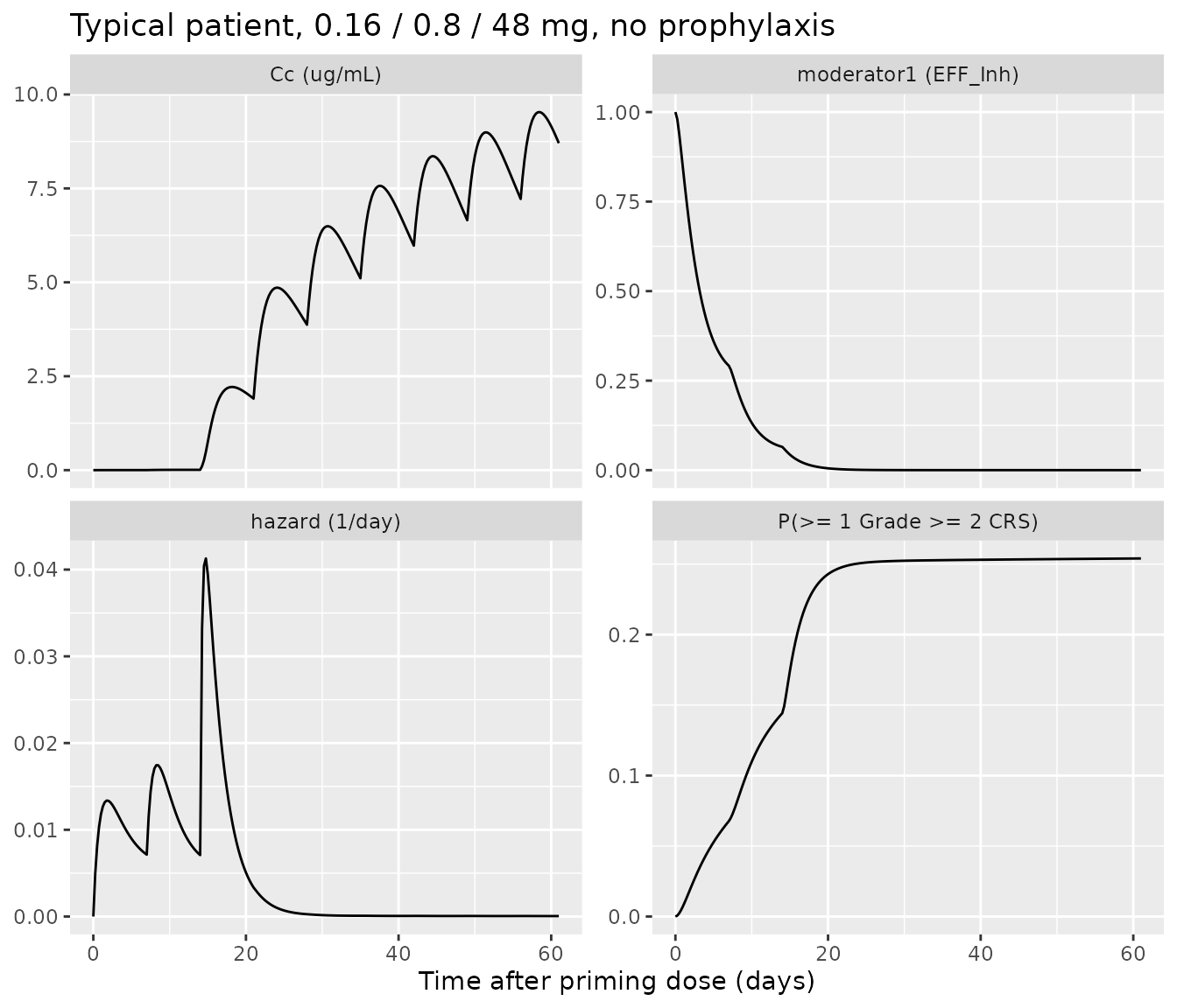
Replicating Figure 5: accelerated step-up regimens
Figure 5 prints the model-predicted Grade >= 2 CRS rate (%) in aNHL for every combination of 1-7 days from the priming dose (0.16 mg) to the intermediate dose (0.8 mg) and 1-7 days from the intermediate dose to the first full dose (48 mg), in four subgroups. The paper does not restate the horizon in the Figure 5 caption; the 61-day window of Figure 4 is used, with weekly 48 mg full doses after the first full dose. The packaged model is solved for the typical patient.
# Printed values, Figure 5, read row by row from the top (7 days from
# intermediate dose to first full dose) to the bottom (1 day); within a row,
# 1 to 7 days from priming to intermediate dose.
fig5_printed <- list(
  a = c(32.8, 30, 27.7, 26.4, 25.6, 25.3, 25.2, 34.8, 31.5, 28.8, 27.1, 26.2, 25.7, 25.7,
    38.3, 33.9, 30.7, 28.6, 27.4, 26.8, 26.5, 43.2, 37.8, 33.8, 31.2, 29.4, 28.4, 28.1,
    50.2, 43.5, 38.6, 35, 32.6, 31.2, 30.5, 59.3, 51.4, 45, 40.4, 37.4, 35.4, 34.3,
    70, 61.1, 53.8, 48, 43.8, 41.2, 39.6),
  b = c(14.1, 12.7, 11.6, 11, 10.7, 10.5, 10.5, 15, 13.4, 12.1, 11.4, 10.9, 10.7, 10.7,
    16.8, 14.6, 13.1, 12.1, 11.5, 11.2, 11.1, 19.4, 16.6, 14.6, 13.3, 12.4, 12, 11.8,
    23.3, 19.6, 17, 15.1, 14, 13.3, 13, 29, 24.1, 20.4, 17.9, 16.3, 15.4, 14.8,
    36.8, 30.3, 25.5, 22.1, 19.8, 18.3, 17.5),
  c = c(17.1, 15.2, 13.9, 13, 12.5, 12.2, 12.1, 19.5, 17, 15.2, 14, 13.4, 13, 12.8,
    23.2, 19.8, 17.3, 15.7, 14.8, 14.2, 14, 28.7, 24, 20.4, 18.3, 16.9, 16.2, 15.8,
    36.2, 30, 25.3, 22.2, 20.3, 19.1, 18.6, 46.4, 38.3, 32.1, 27.7, 25, 23.3, 22.5,
    58.5, 49.1, 41.2, 35.2, 31.3, 28.9, 27.4),
  d = c(6.9, 6.1, 5.5, 5.2, 5, 4.9, 4.8, 7.9, 6.9, 6.1, 5.6, 5.3, 5.2, 5.1,
    9.6, 8.1, 7, 6.3, 5.9, 5.7, 5.6, 12.1, 9.9, 8.4, 7.4, 6.8, 6.5, 6.3,
    15.8, 12.7, 10.5, 9.2, 8.3, 7.8, 7.5, 21.2, 16.8, 13.7, 11.6, 10.4, 9.6, 9.3,
    28.5, 22.7, 18.3, 15.3, 13.3, 12.2, 11.5)
)
fig5_panels <- data.frame(
  panel = c("a", "b", "c", "d"),
  panel_label = c("(a) No prior CAR T, no IV fluids nor dexamethasone",
    "(b) Prior CAR T, no IV fluids nor dexamethasone",
    "(c) No prior CAR T, IV fluids and dexamethasone",
    "(d) Prior CAR T, IV fluids and dexamethasone"),
  PRIOR_CART = c(0L, 1L, 0L, 1L),
  proph = c(0L, 0L, 1L, 1L)
)
fig5_ref <- bind_rows(lapply(names(fig5_printed), function(p) {
  expand.grid(x = 1:7, y = 7:1) |>
    mutate(panel = p, printed = fig5_printed[[p]])
}))
fig5_cohort <- fig5_ref |>
  left_join(fig5_panels, by = "panel") |>
  mutate(id = row_number(), WT = 72.8, AGE = 66,
    CONMED_DEXAMETHASONE = proph, CONMED_IV_FLUIDS = proph)
# One subject per cell; each subject has its own step-up timing.
fig5_doses <- bind_rows(lapply(seq_len(nrow(fig5_cohort)), function(i) {
  r <- fig5_cohort[i, ]
  cbind(id = r$id, regimen_doses(c(0, r$x, r$x + r$y), c(0.16, 0.8, 48)))
}))
ev_fig5 <- bind_rows(
  fig5_doses |> mutate(evid = 1L, cmt = "depot"),
  data.frame(id = fig5_cohort$id, time = 61, amt = 0, evid = 0L, cmt = "central")
) |>
  left_join(fig5_cohort |> select(id, WT, AGE, PRIOR_CART, CONMED_DEXAMETHASONE,
    CONMED_IV_FLUIDS), by = "id") |>
  arrange(id, time, desc(evid)) |>
  as.data.frame()

solve_fig5 <- function(model) {
  rxode2::rxSolve(model, events = ev_fig5, returnType = "data.frame") |>
    filter(time == 61) |>
    transmute(id, simulated = 100 * (1 - sur)) |>
    right_join(fig5_cohort, by = "id") |>
    mutate(pct_diff = 100 * (simulated - printed) / printed)
}
fig5_res <- solve_fig5(mod_typ)
#> ℹ omega/sigma items treated as zero: 'etalcl', 'etalq', 'etalvc', 'etalvp', 'etalka', 'etalrbase_target', 'etalkss', 'etalkint', 'etaRUV'
#> Warning: multi-subject simulation without without 'omega'

fig5_summary <- fig5_res |>
  group_by(panel_label) |>
  summarise(
    `Median % difference` = round(median(pct_diff), 1),
    `90th pct of |% difference|` = round(quantile(abs(pct_diff), 0.9), 1),
    `Standard regimen (7, 7): printed` = printed[x == 7 & y == 7],
    `Standard regimen (7, 7): simulated` = round(simulated[x == 7 & y == 7], 1),
    `Fastest (1, 1): printed` = printed[x == 1 & y == 1],
    `Fastest (1, 1): simulated` = round(simulated[x == 1 & y == 1], 1),
    .groups = "drop"
  ) |>
  rename(Subgroup = panel_label)
knitr::kable(fig5_summary, caption = "Packaged model vs the rates printed in Figure 5 of Li 2026 (Grade >= 2 CRS, %).")| Subgroup | Median % difference | 90th pct of |% difference| | Standard regimen (7, 7): printed | Standard regimen (7, 7): simulated | Fastest (1, 1): printed | Fastest (1, 1): simulated |
|---|---|---|---|---|---|---|
| (a) No prior CAR T, no IV fluids nor dexamethasone | 1.3 | 5.5 | 25.2 | 25.4 | 70.0 | 70.7 |
| (b) Prior CAR T, no IV fluids nor dexamethasone | 1.6 | 6.7 | 10.5 | 10.6 | 36.8 | 37.4 |
| (c) No prior CAR T, IV fluids and dexamethasone | 7.8 | 11.0 | 12.1 | 13.1 | 58.5 | 58.8 |
| (d) Prior CAR T, IV fluids and dexamethasone | 8.6 | 11.7 | 4.8 | 5.2 | 28.5 | 28.7 |
fig5_res |>
  ggplot(aes(factor(x), factor(y), fill = simulated)) +
  geom_tile(colour = "white") +
  geom_text(aes(label = sprintf("%.1f\n(%.1f)", simulated, printed)), size = 2.4) +
  scale_fill_gradient(low = "#d9f0a3", high = "#f768a1", name = "Simulated %") +
  facet_wrap(~panel_label, ncol = 2) +
  labs(x = "Time from priming dose to intermediate dose (days)",
    y = "Time from intermediate dose to first full dose (days)",
    caption = "Cell text: packaged model (printed Figure 5 value in parentheses).")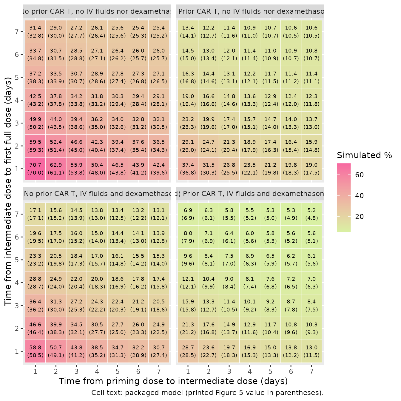
Replicates Figure 5 of Li 2026. The packaged model reproduces all 196 printed rates: panels (a) and (b) within a median of about 1.5%, panels (c) and (d), which carry the prophylaxis effect on S50, about 8% high. The residual is consistent with the paper’s simulation design (virtual patients with sampled body weight and age, and parameter sets drawn from the estimation uncertainty), which a typical-patient solve does not reproduce.
fig5_gate <- fig5_res |>
  group_by(panel) |>
  summarise(med = median(pct_diff), q90 = quantile(abs(pct_diff), 0.9))
fig5_gate
#> # A tibble: 4 × 3
#>   panel   med   q90
#>   <chr> <dbl> <dbl>
#> 1 a      1.30  5.47
#> 2 b      1.59  6.65
#> 3 c      7.83 11.0
#> 4 d      8.62 11.7
stopifnot(
  # A transcription error in any hazard parameter or covariate effect moves a
  # whole panel by tens of percent.
  all(abs(fig5_gate$med) < 10),
  all(fig5_gate$q90 < 15)
)
Table 2 versus the abstract
The abstract reports, for “the calibrated model”, a 69.7% reduction in SMAX with prior CAR T cell therapy (0.303-fold) and 2.89-fold and 3.79-fold increases in S50 with one or both prophylaxis measures. Table 2 and the Results text give 0.382, 3.28 and 5.10, and Table 2 is the only complete parameter set the paper prints. Swapping the three abstract coefficients into the packaged model and repeating the Figure 5 comparison shows that Figure 5 was produced with the Table 2 values, so Table 2 is what the package ships.
mod_abstract <- mod_typ |>
  rxode2::ini(
    e_prior_cart_emax = log(0.303),
    e_proph_either_ec50 = log(2.89),
    e_proph_both_ec50 = log(3.79)
  )
#> ℹ change initial estimate of `e_prior_cart_emax` to `-1.19402247347277`
#> ℹ change initial estimate of `e_proph_either_ec50` to `1.06125650212434`
#> ℹ change initial estimate of `e_proph_both_ec50` to `1.33236601909433`
fig5_abstract <- solve_fig5(mod_abstract)
#> ℹ omega/sigma items treated as zero: 'etalcl', 'etalq', 'etalvc', 'etalvp', 'etalka', 'etalrbase_target', 'etalkss', 'etalkint', 'etaRUV'
#> Warning: multi-subject simulation without without 'omega'
abstract_cmp <- bind_rows(
  fig5_res |> mutate(coefficients = "Table 2 (packaged)"),
  fig5_abstract |> mutate(coefficients = "Abstract")
) |>
  group_by(coefficients, panel) |>
  summarise(med = median(pct_diff), .groups = "drop")
abstract_cmp |>
  mutate(med = round(med, 1)) |>
  pivot_wider(names_from = panel, values_from = med) |>
  rename(`Coefficients` = coefficients, `(a)` = a, `(b)` = b, `(c)` = c, `(d)` = d) |>
knitr::kable(caption = "Median % difference from the printed Figure 5 rates, by panel.")| Coefficients | (a) | (b) | (c) | (d) |
|---|---|---|---|---|
| Abstract | 1.3 | -17.7 | 18.9 | -3.4 |
| Table 2 (packaged) | 1.3 | 1.6 | 7.8 | 8.6 |
med_of <- function(coef, p) abstract_cmp$med[abstract_cmp$coefficients == coef & abstract_cmp$panel == p]
stopifnot(
  # Panel (b) isolates the prior-CAR-T effect, panel (c) the both-prophylaxis
  # effect; Table 2 fits both clearly better than the abstract values.
  abs(med_of("Table 2 (packaged)", "b")) < abs(med_of("Abstract", "b")) - 5,
  abs(med_of("Table 2 (packaged)", "c")) < abs(med_of("Abstract", "c")) - 5
)
Virtual cohort
For the population-level figures, virtual patients are built the way the paper describes its simulations: typical PK parameters, with body weight and age drawn from distributions matching the pooled population (Table S1 medians and ranges; the paper reports means and variances it does not print, so a log-normal weight with 18% spread and a normal age with SD 10 years, truncated to the observed ranges, are assumed). 200 virtual patients are reused across every regimen and prophylaxis arm.
set.seed(20261001)
n_vp <- 200L
vp <- data.frame(
  vp = seq_len(n_vp),
  WT = pmin(pmax(72.8 * exp(rnorm(n_vp, 0, 0.18)), 46), 109.4),
  AGE = pmin(pmax(rnorm(n_vp, 66, 10), 33), 83)
)
summary(vp[, c("WT", "AGE")])
#>        WT              AGE
#>  Min.   : 46.00   Min.   :37.70
#>  1st Qu.: 65.10   1st Qu.:60.89
#>  Median : 73.46   Median :66.80
#>  Mean   : 74.30   Mean   :67.26
#>  3rd Qu.: 80.96   3rd Qu.:73.97
#>  Max.   :109.40   Max.   :83.00
Replicating Figure 4: step-up regimens and prophylaxis
Figure 4 shows the probability of at least one Grade >= 2 CRS event within 61 days for three 2-SUD regimens in aNHL and for 2-SUD vs 3-SUD regimens in iNHL, under the three prophylaxis categories, for patients without prior CAR T cell therapy. The point estimates below were read from Figure 4 by the maintainers (about +/- 0.01). Hazard parameters do not depend on disease type, so aNHL and iNHL differ only in the regimens simulated.
fig4_arms <- tribble(
  ~indication, ~regimen, ~times, ~amts,
  "aNHL", "0.16 / 0.8 / 48 / 48 mg", c(0, 7, 14), c(0.16, 0.8, 48),
  "aNHL", "0.32 / 1.6 / 48 / 48 mg", c(0, 7, 14), c(0.32, 1.6, 48),
  "aNHL", "0.64 / 3 / 48 / 48 mg", c(0, 7, 14), c(0.64, 3, 48),
  "iNHL", "0.16 / 0.8 / 48 / 48 mg", c(0, 7, 14), c(0.16, 0.8, 48),
  "iNHL", "0.16 / 0.8 / 6 / 48 mg", c(0, 7, 14, 21), c(0.16, 0.8, 6, 48),
  "iNHL", "0.16 / 0.8 / 3 / 48 mg", c(0, 7, 14, 21), c(0.16, 0.8, 3, 48)
) |>
  mutate(arm_regimen = row_number())
proph_levels <- tribble(
  ~prophylaxis, ~CONMED_DEXAMETHASONE, ~CONMED_IV_FLUIDS,
  "No IV fluids or dexamethasone", 0L, 0L,
  "IV fluids or dexamethasone", 1L, 0L,
  "IV fluids and dexamethasone", 1L, 1L
)
fig4_cohort <- tidyr::crossing(fig4_arms |> select(indication, regimen, arm_regimen),
  proph_levels, vp) |>
  mutate(id = row_number(), PRIOR_CART = 0L)
fig4_doses <- bind_rows(lapply(seq_len(nrow(fig4_arms)), function(i) {
  cbind(arm_regimen = i, regimen_doses(fig4_arms$times[[i]], fig4_arms$amts[[i]]))
}))
ev_fig4 <- bind_rows(
  inner_join(fig4_cohort, fig4_doses, by = "arm_regimen", relationship = "many-to-many") |>
    mutate(evid = 1L, cmt = "depot"),
  fig4_cohort |> mutate(time = 61, amt = 0, evid = 0L, cmt = "central")
) |>
  arrange(id, time, desc(evid)) |>
  as.data.frame()
sim_fig4 <- rxode2::rxSolve(mod_typ, events = ev_fig4,
  keep = c("indication", "regimen", "prophylaxis"), returnType = "data.frame") |>
  filter(time == 61)
#> ℹ omega/sigma items treated as zero: 'etalcl', 'etalq', 'etalvc', 'etalvp', 'etalka', 'etalrbase_target', 'etalkss', 'etalkint', 'etaRUV'
#> Warning: multi-subject simulation without without 'omega'

fig4_digitised <- tribble(
  ~indication, ~regimen, ~prophylaxis, ~published,
  "aNHL", "0.16 / 0.8 / 48 / 48 mg", "No IV fluids or dexamethasone", 0.245,
  "aNHL", "0.16 / 0.8 / 48 / 48 mg", "IV fluids or dexamethasone", 0.145,
  "aNHL", "0.16 / 0.8 / 48 / 48 mg", "IV fluids and dexamethasone", 0.12,
  "aNHL", "0.32 / 1.6 / 48 / 48 mg", "No IV fluids or dexamethasone", 0.225,
  "aNHL", "0.32 / 1.6 / 48 / 48 mg", "IV fluids or dexamethasone", 0.137,
  "aNHL", "0.32 / 1.6 / 48 / 48 mg", "IV fluids and dexamethasone", 0.108,
  "aNHL", "0.64 / 3 / 48 / 48 mg", "No IV fluids or dexamethasone", 0.24,
  "aNHL", "0.64 / 3 / 48 / 48 mg", "IV fluids or dexamethasone", 0.132,
  "aNHL", "0.64 / 3 / 48 / 48 mg", "IV fluids and dexamethasone", 0.11,
  "iNHL", "0.16 / 0.8 / 48 / 48 mg", "No IV fluids or dexamethasone", 0.28,
  "iNHL", "0.16 / 0.8 / 48 / 48 mg", "IV fluids or dexamethasone", 0.165,
  "iNHL", "0.16 / 0.8 / 48 / 48 mg", "IV fluids and dexamethasone", 0.145,
  "iNHL", "0.16 / 0.8 / 6 / 48 mg", "No IV fluids or dexamethasone", 0.24,
  "iNHL", "0.16 / 0.8 / 6 / 48 mg", "IV fluids or dexamethasone", 0.12,
  "iNHL", "0.16 / 0.8 / 6 / 48 mg", "IV fluids and dexamethasone", 0.095,
  "iNHL", "0.16 / 0.8 / 3 / 48 mg", "No IV fluids or dexamethasone", 0.25,
  "iNHL", "0.16 / 0.8 / 3 / 48 mg", "IV fluids or dexamethasone", 0.115,
  "iNHL", "0.16 / 0.8 / 3 / 48 mg", "IV fluids and dexamethasone", 0.09
)
fig4_res <- sim_fig4 |>
  group_by(indication, regimen, prophylaxis) |>
  summarise(simulated = mean(1 - sur), .groups = "drop") |>
  left_join(fig4_digitised, by = c("indication", "regimen", "prophylaxis")) |>
  mutate(diff = simulated - published)

fig4_res |>
  mutate(simulated = round(simulated, 3), diff = round(diff, 3)) |>
  rename(Indication = indication, Regimen = regimen, Prophylaxis = prophylaxis,
    `Simulated P(>= 1 event, 61 d)` = simulated,
    `Figure 4 (digitised)` = published, Difference = diff) |>
knitr::kable(caption = "Probability of at least one Grade >= 2 CRS event within 61 days, no prior CAR T cell therapy.")| Indication | Regimen | Prophylaxis | Simulated P(>= 1 event, 61 d) | Figure 4 (digitised) | Difference |
|---|---|---|---|---|---|
| aNHL | 0.16 / 0.8 / 48 / 48 mg | IV fluids and dexamethasone | 0.131 | 0.120 | 0.011 |
| aNHL | 0.16 / 0.8 / 48 / 48 mg | IV fluids or dexamethasone | 0.156 | 0.145 | 0.011 |
| aNHL | 0.16 / 0.8 / 48 / 48 mg | No IV fluids or dexamethasone | 0.254 | 0.245 | 0.009 |
| aNHL | 0.32 / 1.6 / 48 / 48 mg | IV fluids and dexamethasone | 0.101 | 0.108 | -0.007 |
| aNHL | 0.32 / 1.6 / 48 / 48 mg | IV fluids or dexamethasone | 0.127 | 0.137 | -0.010 |
| aNHL | 0.32 / 1.6 / 48 / 48 mg | No IV fluids or dexamethasone | 0.236 | 0.225 | 0.011 |
| aNHL | 0.64 / 3 / 48 / 48 mg | IV fluids and dexamethasone | 0.095 | 0.110 | -0.015 |
| aNHL | 0.64 / 3 / 48 / 48 mg | IV fluids or dexamethasone | 0.124 | 0.132 | -0.008 |
| aNHL | 0.64 / 3 / 48 / 48 mg | No IV fluids or dexamethasone | 0.252 | 0.240 | 0.012 |
| iNHL | 0.16 / 0.8 / 3 / 48 mg | IV fluids and dexamethasone | 0.081 | 0.090 | -0.009 |
| iNHL | 0.16 / 0.8 / 3 / 48 mg | IV fluids or dexamethasone | 0.106 | 0.115 | -0.009 |
| iNHL | 0.16 / 0.8 / 3 / 48 mg | No IV fluids or dexamethasone | 0.222 | 0.250 | -0.028 |
| iNHL | 0.16 / 0.8 / 48 / 48 mg | IV fluids and dexamethasone | 0.131 | 0.145 | -0.014 |
| iNHL | 0.16 / 0.8 / 48 / 48 mg | IV fluids or dexamethasone | 0.156 | 0.165 | -0.009 |
| iNHL | 0.16 / 0.8 / 48 / 48 mg | No IV fluids or dexamethasone | 0.254 | 0.280 | -0.026 |
| iNHL | 0.16 / 0.8 / 6 / 48 mg | IV fluids and dexamethasone | 0.079 | 0.095 | -0.016 |
| iNHL | 0.16 / 0.8 / 6 / 48 mg | IV fluids or dexamethasone | 0.105 | 0.120 | -0.015 |
| iNHL | 0.16 / 0.8 / 6 / 48 mg | No IV fluids or dexamethasone | 0.222 | 0.240 | -0.018 |
fig4_res |>
  pivot_longer(c(simulated, published), names_to = "source", values_to = "p") |>
  mutate(source = recode(source, simulated = "Packaged model", published = "Figure 4 (digitised)")) |>
  ggplot(aes(p, regimen, colour = prophylaxis, shape = source)) +
  geom_point(size = 2.5, position = position_dodge(width = 0.5)) +
  scale_shape_manual(values = c(1, 16)) +
  facet_wrap(~indication, ncol = 1, scales = "free_y") +
  labs(x = "Probability of at least one Grade >= 2 CRS event within 61 days",
    y = NULL, colour = NULL, shape = NULL) +
  theme(legend.position = "bottom", legend.box = "vertical")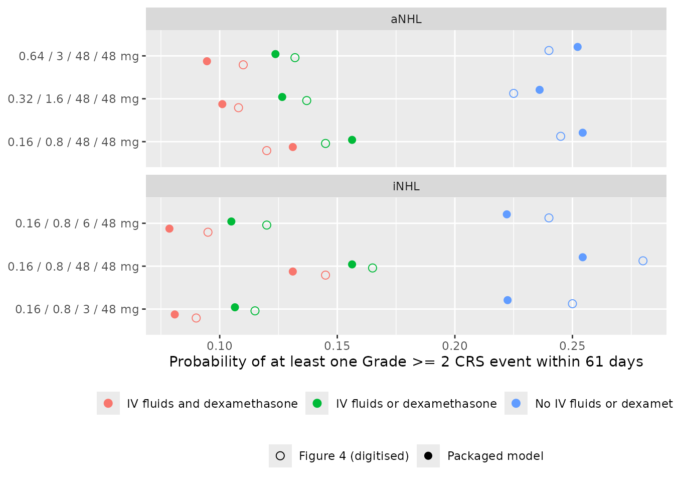
Replicates Figure 4 of Li 2026. All 18 arms land within 0.03 of the published point, and the packaged model reproduces the paper’s conclusions: prophylaxis lowers the risk under every regimen, the two alternative aNHL regimens change it little, and the 3-SUD regimens lower it in iNHL. The largest differences are in iNHL without prophylaxis (about -0.03). Figure 4 plots the iNHL 0.16 / 0.8 / 48 mg arms 0.02-0.04 above the identical aNHL arms although the hazard parameters do not depend on disease type; the paper’s iNHL simulations may have used iNHL-specific covariate distributions, which this model (whose PK covariates are body weight and age only) does not reproduce.
stopifnot(
  abs(median(fig4_res$diff)) < 0.02,
  max(abs(fig4_res$diff)) < 0.06,
  # Direction checks the paper draws its conclusions from: prophylaxis lowers
  # risk in every regimen, and 3-SUD beats 2-SUD in iNHL.
  all(with(fig4_res |> select(indication, regimen, prophylaxis, simulated) |>
    pivot_wider(names_from = prophylaxis, values_from = simulated),
  `No IV fluids or dexamethasone` > `IV fluids or dexamethasone` &
    `IV fluids or dexamethasone` > `IV fluids and dexamethasone`))
)
Replicating Figure 3: the 2-SUD dose grid
Figure 3 maps the probability of at least one Grade >= 2 CRS event over a grid of priming and intermediate doses (aNHL, no IV fluids or dexamethasone, 2-SUD with full 48 mg doses from day 15). Twenty log-spaced doses from 0.01 to 10 mg are used on each axis, matching the plotted range, for the typical patient.
dose_grid <- signif(10^seq(-2, 1, length.out = 20), 3)
fig3_cohort <- expand.grid(priming = dose_grid, intermediate = dose_grid) |>
  mutate(id = row_number(), WT = 72.8, AGE = 66, PRIOR_CART = 0L,
    CONMED_DEXAMETHASONE = 0L, CONMED_IV_FLUIDS = 0L)
fig3_doses <- bind_rows(lapply(seq_len(nrow(fig3_cohort)), function(i) {
  cbind(id = i, regimen_doses(c(0, 7, 14),
    c(fig3_cohort$priming[i], fig3_cohort$intermediate[i], 48)))
}))
ev_fig3 <- bind_rows(
  fig3_doses |> mutate(evid = 1L, cmt = "depot"),
  data.frame(id = fig3_cohort$id, time = 61, amt = 0, evid = 0L, cmt = "central")
) |>
  left_join(fig3_cohort |> select(-priming, -intermediate), by = "id") |>
  arrange(id, time, desc(evid)) |>
  as.data.frame()
fig3_res <- rxode2::rxSolve(mod_typ, events = ev_fig3, returnType = "data.frame") |>
  filter(time == 61) |>
  transmute(id, p = 1 - sur) |>
  left_join(fig3_cohort |> select(id, priming, intermediate), by = "id") |>
  mutate(band = cut(p, breaks = c(0, 0.15, 0.25, 0.35, 0.45, 0.55, 0.65, 1)))
#> ℹ omega/sigma items treated as zero: 'etalcl', 'etalq', 'etalvc', 'etalvp', 'etalka', 'etalrbase_target', 'etalkss', 'etalkint', 'etaRUV'
#> Warning: multi-subject simulation without without 'omega'

ggplot(fig3_res, aes(priming, intermediate, fill = band)) +
  geom_tile() +
  scale_x_log10() +
  scale_y_log10() +
  scale_fill_viridis_d(name = "P(>= 1 Grade >= 2 CRS)", drop = FALSE) +
  annotate("point", x = c(0.16, 0.32, 0.64), y = c(0.8, 1.6, 3), colour = "red",
    shape = c(16, 17, 15), size = 2.5) +
  labs(x = "Priming dose (mg)", y = "Intermediate dose (mg)")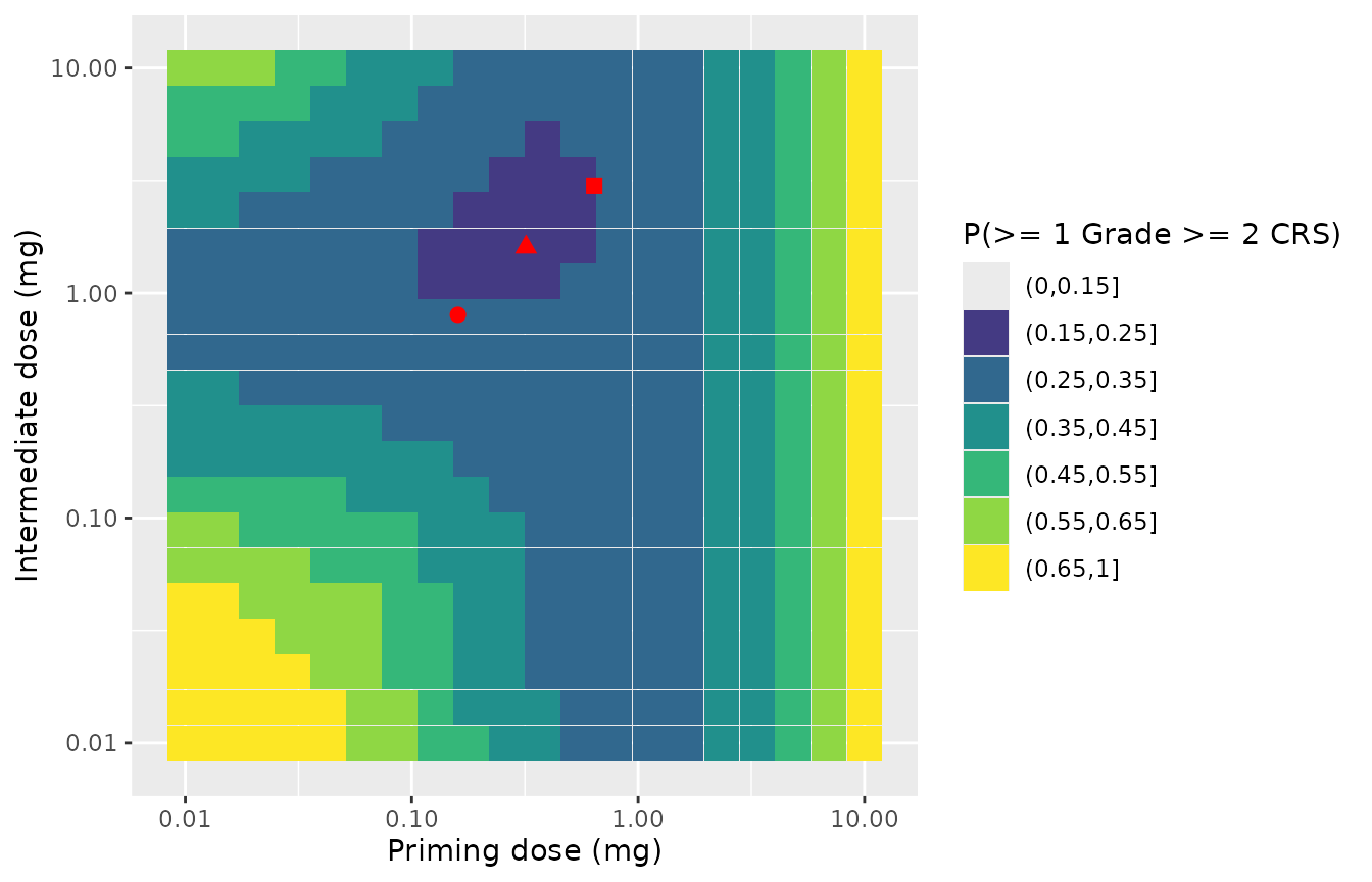
Replicates the shape of Figure 3 of Li 2026, but not its levels. As in the paper, the lowest risk lies in a valley around priming 0.1-1 mg and intermediate about 1-3 mg, which contains the three marked regimens; very low step-up doses build little tolerance before the full dose, and high priming doses produce a large stimulation before tolerance has built up. Away from that valley, the packaged model is about one colour band (0.1) higher than Figure 3: 0.78 vs (0.55, 0.65] at 0.01 / 0.01 mg and 0.65 vs (0.45, 0.55] at a 10 mg priming dose, and the darkest band (<= 0.25) covers only a few grid cells rather than a broad region. The paper used Figure 3 to choose the alternative regimens (0.32 / 1.6 and 0.64 / 3 mg) that were then tested in the dose-optimisation part of EPCORE NHL-1, and it describes Figure 4, not Figure 3, as “based on the final model – including data from the optimization arm”. Figure 3 was therefore most likely produced with an earlier fit, before the optimisation data existed. The packaged Table 2 values reproduce Figures 4 and 5, so nothing is adjusted to match Figure 3.
p_at <- function(pr, im) {
  fig3_res$p[which.min(abs(log(fig3_res$priming / pr)) + abs(log(fig3_res$intermediate / im)))]
}
fig3_check <- data.frame(
  point = c("0.01 / 0.01 mg (bottom-left corner)", "10 / 1 mg (right edge)",
    "grid minimum", "0.16 / 0.8 mg"),
  simulated = c(p_at(0.01, 0.01), p_at(10, 1), min(fig3_res$p), p_at(0.16, 0.8)),
  figure_3_band = c("(0.55, 0.65]", "(0.45, 0.55]", "(0.15, 0.25]", "(0.15, 0.25]")
)
knitr::kable(fig3_check, digits = 3)| point | simulated | figure_3_band |
|---|---|---|
| 0.01 / 0.01 mg (bottom-left corner) | 0.778 | (0.55, 0.65] |
| 10 / 1 mg (right edge) | 0.653 | (0.45, 0.55] |
| grid minimum | 0.235 | (0.15, 0.25] |
| 0.16 / 0.8 mg | 0.253 | (0.15, 0.25] |
fig3_min <- fig3_res[which.min(fig3_res$p), ]
fig3_min
#>      id        p priming intermediate        band
#> 290 290 0.235189   0.264         1.62 (0.15,0.25]
stopifnot(
  # Shape: the minimum lies in the valley that holds the marked regimens ...
  fig3_min$priming > 0.1, fig3_min$priming < 1,
  fig3_min$intermediate > 0.5, fig3_min$intermediate < 5,
  min(fig3_res$p) > 0.15, min(fig3_res$p) < 0.27,
  # ... the approved and alternative regimens sit near that minimum ...
  p_at(0.16, 0.8) - min(fig3_res$p) < 0.03,
  p_at(0.32, 1.6) - min(fig3_res$p) < 0.03,
  p_at(0.64, 3) - min(fig3_res$p) < 0.03,
  # ... and both extremes of the grid are much riskier.
  p_at(0.01, 0.01) > 0.5,
  p_at(10, 1) > 0.45
)
Pooled-population check against Figure 2
Figure 2 compares the observed and simulated time to the first Grade
>= 2 CRS event and the number of events per patient in all 600
patients. The observed cohort received many different regimens,
including the dose-escalation doses, which the paper does not tabulate,
so this is an approximate check: the 200 virtual patients receive the
prior-CAR-T and prophylaxis mix of Table 1, the 2-SUD regimen if aNHL or
in the expansion part and the 3-SUD (0.16 / 0.8 / 3 / 48 mg) regimen for
the iNHL patients of the dose-optimisation part. Because the hazard does
not depend on the event history, the number of events by day 61 is
Poisson with mean cumhaz(61), so the expected count
distribution is computed exactly rather than by sampling.
set.seed(20261002)
pooled <- vp |>
  mutate(
    id = vp,
    PRIOR_CART = rbinom(n_vp, 1, 125 / 600),
    proph = sample(c("none", "ivf", "dex", "both"), n_vp, replace = TRUE,
      prob = c(373, 30, 91, 106) / 600),
    CONMED_DEXAMETHASONE = as.integer(proph %in% c("dex", "both")),
    CONMED_IV_FLUIDS = as.integer(proph %in% c("ivf", "both")),
    # 81 of 600 were iNHL in the dose-optimisation part (Table 1).
    sud3 = rbinom(n_vp, 1, 81 / 600)
  )
pooled_doses <- bind_rows(
  cbind(sud3 = 0L, regimen_doses(c(0, 7, 14), c(0.16, 0.8, 48))),
  cbind(sud3 = 1L, regimen_doses(c(0, 7, 14, 21), c(0.16, 0.8, 3, 48)))
)
ev_pooled <- bind_rows(
  inner_join(pooled, pooled_doses, by = "sud3", relationship = "many-to-many") |>
    mutate(evid = 1L, cmt = "depot"),
  tidyr::crossing(pooled, time = 0:61) |> mutate(amt = 0, evid = 0L, cmt = "central")
) |>
  select(id, time, amt, evid, cmt, WT, AGE, PRIOR_CART, CONMED_DEXAMETHASONE, CONMED_IV_FLUIDS) |>
  arrange(id, time, desc(evid)) |>
  as.data.frame()
sim_pooled <- rxode2::rxSolve(mod_typ, events = ev_pooled, returnType = "data.frame")
#> ℹ omega/sigma items treated as zero: 'etalcl', 'etalq', 'etalvc', 'etalvp', 'etalka', 'etalrbase_target', 'etalkss', 'etalkint', 'etaRUV'
#> Warning: multi-subject simulation without without 'omega'

km_sim <- sim_pooled |>
  group_by(time) |>
  summarise(sur = mean(sur), .groups = "drop")
ggplot(km_sim, aes(time, sur)) +
  geom_line(colour = "#d95f02", linewidth = 1) +
  coord_cartesian(ylim = c(0, 1)) +
  labs(x = "Time (days after priming dose)",
    y = "Probability of no Grade >= 2 CRS event")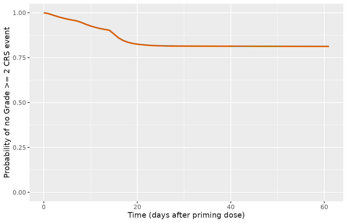
h61 <- sim_pooled$cumhaz[sim_pooled$time == 61]
expected_counts <- data.frame(events = 0:4) |>
  rowwise() |>
  mutate(`Expected patients (of 600)` = round(600 * mean(dpois(events, h61)), 1)) |>
  ungroup()
knitr::kable(expected_counts, caption = "Expected number of patients by number of Grade >= 2 CRS events within 61 days, scaled to 600.")| events | Expected patients (of 600) |
|---|---|
| 0 | 487.6 |
| 1 | 99.2 |
| 2 | 12.0 |
| 3 | 1.1 |
| 4 | 0.1 |
p_free_61 <- km_sim$sur[km_sim$time == 61]
p_free_61
#> [1] 0.8127143
stopifnot(
  # Figure 2 top panel: the observed and simulated event-free fraction
  # plateaus near 0.80 by day 30-61 (read from the figure).
  p_free_61 > 0.72, p_free_61 < 0.88,
  # Figure 2 bottom panel: about 470 patients with no event and about 100
  # with one; very few with three or more.
  expected_counts$`Expected patients (of 600)`[1] > 430,
  expected_counts$`Expected patients (of 600)`[4] < 10
)
Replicates Figure 2 of Li 2026 approximately: the simulated event-free probability falls mainly between the first full dose (day 15) and day 30 and plateaus near 0.8 (0.81 at day 61). The expected numbers of patients with 0, 1 and 2 events (about 488, 99 and 12 of 600) compare with roughly 470, 105 and 20 in the bottom panel; this approximate cohort has slightly fewer patients with repeated events.
PKNCA: exposure delivered by the step-up doses
The CRS paper reports no NCA values. PKNCA is used here to summarise the epcoritamab exposure (free plasma concentration, the hazard driver) during the priming, intermediate and first full-dose weeks of the approved 2-SUD regimen in the virtual cohort, and the mean hazard in each week, which shows how tolerance from the low step-up doses limits the hazard after the first full dose.
ev_nca <- build_events(
  vp |> mutate(id = vp, PRIOR_CART = 0L, CONMED_DEXAMETHASONE = 0L,
    CONMED_IV_FLUIDS = 0L, treatment = "0.16 / 0.8 / 48 mg"),
  regimen_doses(c(0, 7, 14), c(0.16, 0.8, 48), horizon = 21),
  seq(0, 21, by = 0.25)
)
sim_nca <- rxode2::rxSolve(mod_typ, events = ev_nca, keep = "treatment",
  returnType = "data.frame")
#> ℹ omega/sigma items treated as zero: 'etalcl', 'etalq', 'etalvc', 'etalvp', 'etalka', 'etalrbase_target', 'etalkss', 'etalkint', 'etaRUV'
#> Warning: multi-subject simulation without without 'omega'

nca_conc <- sim_nca |>
  filter(!is.na(Cc)) |>
  select(id, time, Cc, treatment)
nca_dose <- ev_nca |>
  filter(evid == 1, time <= 14) |>
  select(id, time, amt, treatment)
nca_intervals <- data.frame(
  start = c(0, 7, 14), end = c(7, 14, 21),
  cmax = TRUE, tmax = TRUE, auclast = TRUE
)
conc_obj <- PKNCA::PKNCAconc(nca_conc, Cc ~ time | treatment + id)
dose_obj <- PKNCA::PKNCAdose(nca_dose, amt ~ time | treatment + id)
nca_res <- PKNCA::pk.nca(PKNCA::PKNCAdata(conc_obj, dose_obj, intervals = nca_intervals))
nca_tab <- as.data.frame(nca_res$result) |>
  mutate(week = factor(start, levels = c(0, 7, 14),
    labels = c("Priming 0.16 mg (days 0-7)", "Intermediate 0.8 mg (days 7-14)",
      "First full 48 mg (days 14-21)"))) |>
  group_by(week, PPTESTCD) |>
  summarise(median = signif(median(PPORRES), 3), .groups = "drop") |>
  pivot_wider(names_from = PPTESTCD, values_from = median)

hazard_week <- sim_nca |>
  mutate(week = cut(time, c(0, 7, 14, 21), include.lowest = TRUE,
    labels = levels(nca_tab$week))) |>
  group_by(week) |>
  summarise(mean_hazard = signif(mean(hazard), 3), .groups = "drop")

nca_tab |>
  left_join(hazard_week, by = "week") |>
  rename(Week = week, `Cmax (ug/mL)` = cmax, `Tmax (day)` = tmax,
    `AUClast (ug*day/mL)` = auclast, `Mean hazard (1/day)` = mean_hazard) |>
knitr::kable(caption = "Median free-epcoritamab NCA by step-up week (PKNCA) and the cohort-mean Grade >= 2 CRS hazard.")| Week | AUClast (ug*day/mL) | Cmax (ug/mL) | Tmax (day) | Mean hazard (1/day) |
|---|---|---|---|---|
| Priming 0.16 mg (days 0-7) | 0.00792 | 0.00139 | 5.25 | 0.00976 |
| Intermediate 0.8 mg (days 7-14) | 0.04960 | 0.00836 | 5.00 | 0.01220 |
| First full 48 mg (days 14-21) | 11.70000 | 2.19000 | 4.25 | 0.01800 |
stopifnot(
  # The 48 mg full dose raises Cmax by three orders of magnitude over the
  # priming dose ...
  nca_tab$cmax[3] > 300 * nca_tab$cmax[1],
  # ... but, because tolerance has built up, the mean hazard rises far less.
  hazard_week$mean_hazard[3] < 3 * hazard_week$mean_hazard[1]
)
Free-epcoritamab Cmax rises more than a thousand-fold from the priming week to the first full-dose week, while the mean hazard rises less than two-fold: by the time the full dose arrives, the low step-up doses have already pushed the tolerance pool far below 1.
Model self-consistency
The cumulative hazard state must equal the time integral of the hazard, and without drug the tolerance pool must stay at 1 and the hazard at 0.
fine <- build_events(typical_patient, sud2, seq(0, 61, by = 0.01))
sim_fine <- rxode2::rxSolve(mod_typ, events = fine, returnType = "data.frame")
#> ℹ omega/sigma items treated as zero: 'etalcl', 'etalq', 'etalvc', 'etalvp', 'etalka', 'etalrbase_target', 'etalkss', 'etalkint', 'etaRUV'
trap <- sum(diff(sim_fine$time) * (head(sim_fine$hazard, -1) + tail(sim_fine$hazard, -1)) / 2)
rel_err <- abs(trap - tail(sim_fine$cumhaz, 1)) / tail(sim_fine$cumhaz, 1)
rel_err
#> [1] 7.801493e-06

no_drug <- rxode2::rxSolve(mod_typ,
  events = build_events(typical_patient, data.frame(time = 0, amt = 0), 0:30),
  returnType = "data.frame")
#> ℹ omega/sigma items treated as zero: 'etalcl', 'etalq', 'etalvc', 'etalvp', 'etalka', 'etalrbase_target', 'etalkss', 'etalkint', 'etaRUV'
stopifnot(
  rel_err < 1e-3,
  all(abs(no_drug$moderator1 - 1) < 1e-8),
  all(no_drug$hazard == 0),
  all(sim_fine$moderator1 > 0 & sim_fine$moderator1 <= 1 + 1e-8)
)
Assumptions and deviations
- Table 2 values, not the abstract’s. The abstract’s covariate effects (0.303-fold SMAX with prior CAR T cell therapy; 2.89-fold and 3.79-fold S50 with one or both prophylaxis measures) differ from Table 2 and the Results text (0.382, 3.28, 5.10). Only Table 2 gives a complete parameter set, and the Figure 5 comparison above shows the paper’s own simulations used the Table 2 values. The Results text also refers to the both-prophylaxis coefficient as “theta14”; it is theta13 in Table 2.
-
Driving concentration.
Cpis taken as the free plasma concentrationCcpredicted by the Li 2025 QSS-TMDD model, the quantity that model was fitted to. Driving the hazard with the total (free + bound) concentration instead reproduces Figure 5 much worse (about +30% in panel (a) for the standard regimen), which supports this reading. - PK covariates. The Methods state that simulations varied body weight, age and baseline tumour size; the published Li 2025 final model, embedded here unchanged, has body weight and age as covariates only, so tumour size plays no part. The covariate distributions (log-normal weight, normal age) are assumptions because only medians and ranges are printed.
-
Typical PK values. The paper calibrated the hazard
with individual EBEs and simulated with typical PK parameters; the
figures here use
rxode2::zeroRe(). The Li 2025 PK IIV is kept in the model file so the PK layer can be simulated stochastically; the hazard itself has no random effects (Table 2, all omegas 0). -
Prophylaxis encoding. The paper’s three-level Cycle
1 prophylaxis covariate (neither / IV fluids or dexamethasone / both) is
rebuilt from the two binary columns
CONMED_DEXAMETHASONEandCONMED_IV_FLUIDS, so users give the facts and the model derives the category. The covariate is a per-patient category and applies throughout the simulated period, as in the source. Prednisolone premedication counts as no dexamethasone. - Dosing after the step-up doses. Simulations give full 48 mg doses weekly after the first full dose (Cycle 1-3 schedule). The Figure 5 horizon is not stated in its caption; 61 days, as in Figure 4, is assumed.
-
Unused parameters. Table 2 lists theta8 (prior CAR
T on Kin), theta10 (prior CAR T on S50) and theta11 (NHL-3 study on S50)
at 0; the footnote says these were not used, so they are not in the
model. Disease type and study are recorded under
covariatesDataExcluded. - Figures 2 and 4 are compared against values read from the figures by the maintainers; Figure 5 values are printed in the paper.
- Figure 3 is reproduced in shape but runs about 0.1 higher than the published colour bands away from the low-risk valley. It was most likely produced with a pre-optimisation fit (see the Figure 3 section); the Table 2 parameters are kept as published.