Patritumab deruxtecan (Lee 2023)
Source:vignettes/articles/Lee_2023_patritumab.Rmd
Lee_2023_patritumab.RmdModel and source
- Citation: Lee M, Wang S, Byrne R, Joshi R, Abutarif M, Garimella T, Li L. Integrated Population Pharmacokinetic Analysis of Conjugated and Unconjugated Payload of Patritumab Deruxtecan in Cancer Patients. American Conference on Pharmacometrics (ACoP) 14 Poster, Oct 2023. https://metrumrg.com/wp-content/uploads/2023/11/34023850_ACoP-2023_Pop_PK_Poster_V01-20Oct2023-1.pdf
- Description: Integrated population PK model for the conjugated (anti-HER3-ac-DXd) and unconjugated payload (DXd) of patritumab deruxtecan (HER3-DXd, U3-1402, anti-HER3 antibody-drug conjugate) in adult cancer patients (Lee 2023 ACoP poster). anti-HER3-ac-DXd disposition is a two-compartment model with three parallel elimination pathways from the central compartment: a transient time-decaying linear clearance CL_t(time) = CL_T * exp(-Kdes * time), a non-specific time-dependent linear clearance CL_ns(time) that declines sigmoidally from CL_ss * (1 + Emax) at time = 0 to CL_ss at infinity via a Hill function CL_ns(time) = CL_ss * (1 + Emax * T50^hill / (T50^hill + time^hill)), and a Michaelis-Menten saturable clearance CL_mm = Vmax / (Km + Cc). DXd is a one-compartment model with parallel linear and Michaelis-Menten elimination; its formation rate equals the sum of the three anti-HER3-ac-DXd elimination rates each scaled by a dimensionless fractional-conversion factor Frac_ns / Frac_t / Frac_mm (Frac_ns fixed at 1 as the identifiability anchor).
- Article: Lee 2023 ACoP 14 Poster (Metrum Research Group)
This is an ACoP 14 (October 2023) conference poster developed by
Daiichi Sankyo and Metrum Research Group. It is distinct from
Lu_2022_patritumab (peer-reviewed J Clin Pharmacol 2023),
which used a different structural form (linear + Michaelis-Menten
anti-HER3-ac-DXd clearance with a within-cycle DAR-modulated first-order
DXd release rate) on a 425-subject cohort spanning studies J101 / U102 /
U202.
Population
The Lee 2023 popPK analysis pooled 401 cancer patients from two Phase 1 / 2 studies of patritumab deruxtecan (HER3-DXd, U3-1402): 182 HER3-expressing breast-cancer patients from U31402-A-J101 (100% female, 78% Asian) and 219 EGFR-mutated NSCLC patients from U31402-A-U102 (63.5% female, 47% Asian). Median age 60 years (range 29 - 83), median body weight 57.4 kg (range 32.4 - 113), median baseline serum albumin 39 g/L, median eGFR 92 mL/min/1.73 m^2 (Lee 2023 Tables 2 and 3). The dose range was 1.6 - 8.0 mg/kg IV every 3 weeks (Q3W), with 5.6 mg/kg Q3W selected for further development. The analysis dataset comprised 6,869 anti-HER3-ac-DXd and 6,821 unconjugated-DXd concentrations.
Programmatic access to the population metadata:
str(mod_obj$meta$population, max.level = 1)
#> List of 19
#>  $ species              : chr "human"
#>  $ n_subjects           : int 401
#>  $ n_studies            : int 2
#>  $ n_observations_ac_dxd: int 6869
#>  $ n_observations_dxd   : int 6821
#>  $ age_range            : chr "29 - 83 years (median 60)"
#>  $ age_median           : chr "60 years"
#>  $ weight_range         : chr "32.4 - 113 kg (median 57.4)"
#>  $ weight_median        : chr "57.4 kg (population median; Lee 2023 Figure 6 reference subject is 60 kg)"
#>  $ sex_female_pct       : num 80
#>  $ race_ethnicity       : Named num [1:6] 61.1 32.2 3.5 2.2 0.5 0.5
#>   ..- attr(*, "names")= chr [1:6] "Asian" "White" "Multiple" "Black" ...
#>  $ disease_state        : chr "Advanced or metastatic solid tumors. 182 / 401 (45.4%) breast cancer (HER3-expressing, Study U31402-A-J101); 21"| __truncated__
#>  $ dose_range           : chr "1.6 - 8.0 mg/kg patritumab deruxtecan IV every 3 weeks (Q3W); the Phase 1 dose-escalation NSCLC arm also enroll"| __truncated__
#>  $ regions              : chr "Multi-regional: U31402-A-J101 enrolled in Japan with global expansion; U31402-A-U102 enrolled globally includin"| __truncated__
#>  $ ecog_pct             : Named num [1:3] 52.1 47.9 0
#>   ..- attr(*, "names")= chr [1:3] "0" "1" "2"
#>  $ hepatic_function     : Named num [1:5] 71.8 26.7 0.7 0 0.7
#>   ..- attr(*, "names")= chr [1:5] "Normal" "Mild" "Moderate" "Severe" ...
#>  $ renal_function       : Named num [1:5] 55.1 34.7 10.2 0 0
#>   ..- attr(*, "names")= chr [1:5] "Normal" "Mild" "Moderate" "Severe" ...
#>  $ reference_subject    : chr "Non-Asian female NSCLC patient, age 60, weight 60 kg, ECOG 0, eGFR 90 mL/min/1.73m^2, albumin 40 g/L, baseline "| __truncated__
#>  $ notes                : chr "ACoP 14 (Oct 2023) conference poster. NONMEM v7.5 sequential fit: anti-HER3-ac-DXd base model, then integrated "| __truncated__
Source trace
The per-parameter source location is recorded as an in-file comment
next to each ini() entry in
inst/modeldb/specificDrugs/Lee_2023_patritumab.R. The
summary below consolidates the equation- and parameter-level
provenance.
| Equation / parameter | Value | Source location |
|---|---|---|
central 2-cmt + peripheral1, three
parallel ADC pathways (CL_t, CL_ns, CL_mm) |
n/a | Lee 2023 “Model Schematic”, Figure 1 |
central_dxd 1-cmt, linear + MM elimination |
n/a | Lee 2023 “Model Schematic”, Figure 1 |
cl_t(time) = cl_time_typ * exp(-kdes * time) |
n/a | Lee 2023 Methods: “CL t = CL T * exp(-k des * time)” |
cl_ns(time) = cl_ss * (1 + emax * t50^hill / (t50^hill + time^hill)) |
n/a | Reconstructed from Lee 2023 Table 4 parameter descriptions (CLinf, CLinf,EMAX, T50, gamma) and Results text “initial value at time zero … 0.0217 L/hr … steady state value of 0.0143 L/hr”; 0.0136 * (1 + 0.603) = 0.0218 ~ 0.0217 |
cl_mm = vmax * central / (km + Cc) |
n/a | Lee 2023 Methods: “CLMM = Vmax / (Km + ac-DXd)” |
formation_dxd = fracns * rate_ns + fract * rate_t + fracmm * rate_mm |
n/a | Lee 2023 Methods: “DXd formation was described by Frac ns, Frac t and Frac mm which were the relative fractions of anti-HER3-ac-DXd CLns, CLt, and CLMM, respectively” |
lcl_time (CL_T) |
0.0858 L/hr | Lee 2023 Table 4, exp(theta1) |
lvc (V1) |
2.91 L | Lee 2023 Table 4, exp(theta2) |
lq (Q) |
0.0221 L/hr | Lee 2023 Table 4, exp(theta3) |
lvp (V2) |
3.17 L | Lee 2023 Table 4, exp(theta4) |
lkdes (Kdes) |
0.217 1/hr | Lee 2023 Table 4, exp(theta5) |
lcl_ss (CL_inf) |
0.0136 L/hr | Lee 2023 Table 4, exp(theta6) |
lemaxclns (CLinf,EMAX) |
0.603 | Lee 2023 Table 4, exp(theta7) |
lt50clns (T50) |
1380 hr | Lee 2023 Table 4, exp(theta8) |
lhillclns (gamma) |
3.75 | Lee 2023 Table 4, exp(theta9) |
lvmax |
2.15 nmol/L/hr | Lee 2023 Table 4, exp(theta10) |
lkm |
45.8 nmol/L | Lee 2023 Table 4, exp(theta11) |
lcl_dxd (CL_DXd) |
4.42 L/hr | Lee 2023 Table 5, exp(theta12) |
lvc_dxd (V1_DXd) |
5.96 L | Lee 2023 Table 5, exp(theta13) |
lvmax_dxd |
6.18 nmol/L/hr | Lee 2023 Table 5, exp(theta16) |
lkm_dxd |
0.483 nmol/L | Lee 2023 Table 5, exp(theta17) |
lfracns (Frac_ns) |
1 FIXED | Lee 2023 Table 5, exp(theta18) FIXED |
lfract (Frac_t) |
0.272 | Lee 2023 Table 5, exp(theta21) |
lfracmm (Frac_mm) |
0.272 | Lee 2023 Table 5, exp(theta22) (identical point estimate and 95% CI 0.0670 - 1.11 to theta21) |
e_bc_cl_time |
log(0.896) | Lee 2023 Table 6, exp(theta24) |
e_sld_cl_time |
-0.0758 | Lee 2023 Table 6, theta25 |
e_male_vc |
log(1.18) | Lee 2023 Table 6, exp(theta26) |
e_asian_vc |
log(0.927) | Lee 2023 Table 6, exp(theta27) |
e_male_cl_ss |
log(1.30) | Lee 2023 Table 6, exp(theta28) |
e_asian_cl_ss |
log(1.02) | Lee 2023 Table 6, exp(theta29) |
e_ecog_cl_ss |
log(1.04) | Lee 2023 Table 6, exp(theta30) |
e_bc_cl_ss |
log(0.937) | Lee 2023 Table 6, exp(theta31) |
e_hep_cl_ss |
log(0.906) | Lee 2023 Table 6, exp(theta33) |
e_egfr_cl_ss |
-0.302 | Lee 2023 Table 6, theta34 |
e_alb_cl_ss |
-0.490 | Lee 2023 Table 6, theta35 |
e_sld_kdes |
-0.139 | Lee 2023 Table 6, theta36 |
e_wt_fracns |
0.139 | Lee 2023 Table 6, theta37 |
e_wt_cl (allometric) |
0.343 | Lee 2023 Table 6, theta46 |
e_wt_vc (allometric) |
0.475 | Lee 2023 Table 6, theta47 |
propSd (anti-HER3-ac-DXd) |
sqrt(0.0342) | Lee 2023 Table 7, Sigma(1,1) (CV% 18.5) |
propSd_dxd (DXd) |
sqrt(0.0814) | Lee 2023 Table 7, Sigma(2,2) (CV% 28.5) |
The full IIV block (etalcl_time, etalvc, etalq, etalvp, etalcl_ss, etalt50clns, etalcl_dxd, etalvc_dxd, etalfracns) and the remaining Frac_ns covariate effects map analogously to Lee 2023 Tables 6 and 7.
Virtual cohort
The reference subject defined by Lee 2023 Figure 6 caption is a non-Asian female NSCLC patient with body weight 60 kg, age 60, ECOG 0, eGFR 90 mL/min/1.73 m^2, serum albumin 40 g/L, baseline SLD 6 cm (= 60 mm), and normal hepatic function. We build (a) the typical reference subject for deterministic figures and (b) a 200-subject stochastic cohort matching the pooled population’s covariate distributions (Lee 2023 Tables 2 and 3) for VPC-style plots.
set.seed(20231020)

mw_adc <- 150000   # patritumab molecular weight (g/mol; mAb scaffold)
mw_dxd <- 493.5    # DXd payload molecular weight (g/mol)
mg_per_kg <- 5.6   # selected Phase 2 dose (Lee 2023 Methods)
tau_hr <- 504      # Q3W dosing interval, hours
n_cycles <- 6      # observation horizon (about 18 weeks)

dose_nmol <- function(weight_kg, mg_per_kg = 5.6, mw = mw_adc) {
  weight_kg * mg_per_kg * 1e6 / mw  # mg -> g/mol-equivalent -> nmol
}

# Helper: build one cohort as an event table. cmt = "central" on
# observation rows is the ADC ODE state name; rxode2 returns Cc and
# Cc_dxd at every observation row regardless of which compartment the
# row points at.
make_cohort <- function(cohort_df, t_obs, id_offset = 0L) {
  cohort_df <- cohort_df |>
    dplyr::mutate(id = id_offset + dplyr::row_number(),
                  amt = dose_nmol(WT))
  doses <- cohort_df |>
    dplyr::transmute(id, time = 0, evid = 1L, amt,
                     cmt = "central", ii = tau_hr, addl = n_cycles - 1L,
                     WT, ALB, CRCL, TUMSZ, SEXF, RACE_ASIAN,
                     ECOG_GE1, TUMTP_BREAST, HEPIMP)
  # For each observation time, emit one row per output (dvid 1 = Cc, dvid 2 = Cc_dxd)
  # with cmt set to the ODE state name backing that output (central for Cc,
  # central_dxd for Cc_dxd). rxode2 returns BOTH Cc and Cc_dxd columns regardless
  # of which observation row triggered, but the cmt+dvid pair must be consistent
  # with the model's auto-generated DVID mapping (see
  # known-vignette-failure-patterns.md pattern #5b).
  obs <- tidyr::expand_grid(
    cohort_df |> dplyr::select(id, WT, ALB, CRCL, TUMSZ, SEXF,
                                RACE_ASIAN, ECOG_GE1, TUMTP_BREAST, HEPIMP),
    time = t_obs,
    output = c("Cc", "Cc_dxd")
  ) |>
    dplyr::mutate(
      evid = 0L,
      amt  = NA_real_,
      cmt  = dplyr::if_else(output == "Cc", "central", "central_dxd"),
      dvid = dplyr::if_else(output == "Cc", 1L, 2L),
      ii   = NA_real_,
      addl = NA_integer_
    ) |>
    dplyr::select(-output)
  dplyr::bind_rows(doses |> dplyr::mutate(dvid = NA_integer_), obs) |>
    dplyr::arrange(id, time, dplyr::desc(evid))
}

# (a) Typical reference subject -- single ID, deterministic time grid
ref_df <- tibble::tibble(
  WT = 60, ALB = 40, CRCL = 90, TUMSZ = 60,
  SEXF = 1L, RACE_ASIAN = 0L, ECOG_GE1 = 0L,
  TUMTP_BREAST = 0L, HEPIMP = 0L
)
t_dense <- sort(unique(c(seq(0, tau_hr * n_cycles, by = 6),
                         seq(0, 48, by = 1),
                         seq(48, 168, by = 4))))
events_ref <- make_cohort(ref_df, t_obs = t_dense)

# (b) Stochastic 200-subject cohort, two tumor types per Table 3
n_per_arm <- 100
breast <- tibble::tibble(
  WT = pmax(35, rnorm(n_per_arm, 54, 13)),
  ALB = pmax(20, rnorm(n_per_arm, 38.2, 5.1)),
  CRCL = pmax(35, rnorm(n_per_arm, 98.4, 17.7)),
  TUMSZ = pmax(10, rnorm(n_per_arm, 78.1, 49.8)),  # mm from Lee 2023 Table 2 (SLD in cm * 10)
  SEXF = 1L, RACE_ASIAN = rbinom(n_per_arm, 1, 0.78),
  ECOG_GE1 = rbinom(n_per_arm, 1, 0.275),
  TUMTP_BREAST = 1L,
  HEPIMP = rbinom(n_per_arm, 1, 0.434)  # 41.8% mild + 1.6% moderate (Lee 2023 Table 3)
)
nsclc <- tibble::tibble(
  WT = pmax(35, rnorm(n_per_arm, 64.2, 15)),
  ALB = pmax(20, rnorm(n_per_arm, 38.7, 4.6)),
  CRCL = pmax(35, rnorm(n_per_arm, 82.1, 18.8)),
  TUMSZ = pmax(10, rnorm(n_per_arm, 63.1, 38.7)),
  SEXF = rbinom(n_per_arm, 1, 0.635),
  RACE_ASIAN = rbinom(n_per_arm, 1, 0.47),
  ECOG_GE1 = rbinom(n_per_arm, 1, 0.648),
  TUMTP_BREAST = 0L,
  HEPIMP = rbinom(n_per_arm, 1, 0.142)
)
t_sparse <- sort(unique(c(seq(0, tau_hr * n_cycles, by = 24),
                          seq(0, 48, by = 3))))
events_pop <- dplyr::bind_rows(
  make_cohort(breast, t_sparse, id_offset = 0L)   |> dplyr::mutate(arm = "Breast cancer"),
  make_cohort(nsclc,  t_sparse, id_offset = 100L) |> dplyr::mutate(arm = "NSCLC")
)
stopifnot(!anyDuplicated(unique(events_pop[, c("id", "time", "evid")])))
Simulation
mod <- mod_obj

# Deterministic typical-subject simulation: zero out IIV and residual error.
sim_typ <- rxode2::rxSolve(rxode2::zeroRe(mod), events = events_ref,
                           returnType = "data.frame")
#> ℹ omega/sigma items treated as zero: 'etalcl_time', 'etalvc', 'etalq', 'etalvp', 'etalcl_ss', 'etalt50clns', 'etalcl_dxd', 'etalvc_dxd', 'etalfracns'

# Stochastic 200-subject VPC simulation (covariate-stratified)
sim_pop <- rxode2::rxSolve(mod, events = events_pop,
                           keep = c("arm"),
                           returnType = "data.frame")
Replicate published figures
Figure 2 – Clearance of anti-HER3-ac-DXd over treatment cycles
sim_typ |>
  dplyr::distinct(time, .keep_all = TRUE) |>
  dplyr::transmute(
    time,
    `CL_t`  = cl_t_now,
    `CL_ns` = cl_ns_now,
    `CL_mm (apparent)` = vmax / (km + Cc)  # Vmax/(Km+C) is the per-amount rate constant
  ) |>
  tidyr::pivot_longer(-time, names_to = "pathway", values_to = "CL_L_per_hr") |>
  ggplot(aes(time / 168, CL_L_per_hr, colour = pathway)) +
  geom_line(linewidth = 0.8) +
  scale_y_log10() +
  labs(x = "Time (weeks)", y = "Pathway-specific apparent clearance (L/hr or 1/hr)",
       colour = NULL,
       title = "Time courses of the three anti-HER3-ac-DXd clearance pathways") +
  theme_bw()
Replicates Lee 2023 Figure 2: the three time-varying ADC clearance pathways at the typical reference subject. CL_t decays rapidly within the first dose interval; CL_ns sigmoidally declines from CL_ss * (1 + Emax) at time = 0 to CL_ss by the end of the simulated 18-week horizon; CL_mm tracks the instantaneous anti-HER3-ac-DXd concentration.
Figure 3 – Formation rate of DXd over treatment cycles
sim_typ |>
  dplyr::distinct(time, .keep_all = TRUE) |>
  ggplot(aes(time / 168, formation_dxd)) +
  geom_line(linewidth = 0.8) +
  labs(x = "Time (weeks)", y = "DXd formation rate (nmol/hr)",
       title = "DXd formation rate over treatment cycles") +
  theme_bw()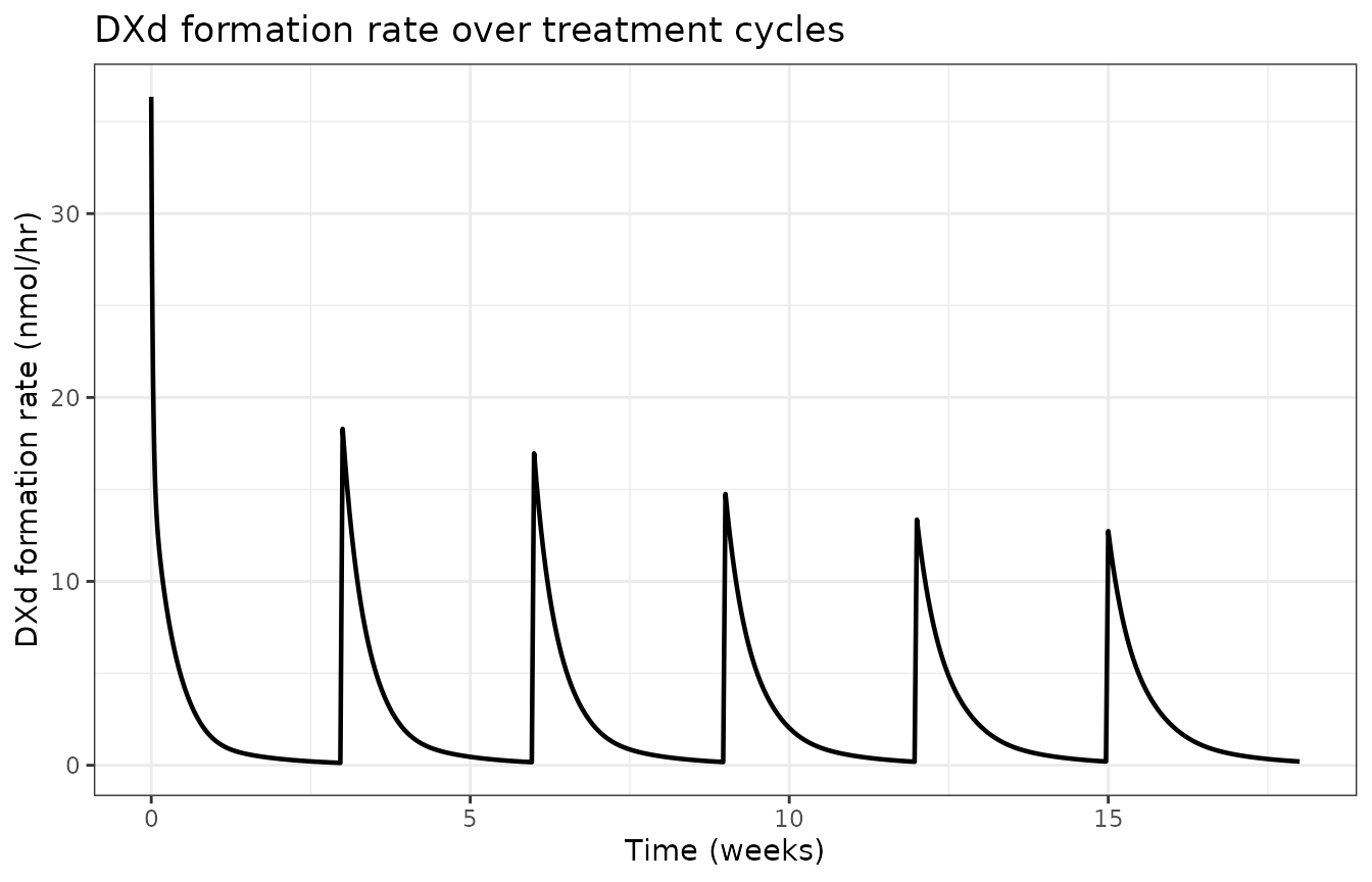
Replicates Lee 2023 Figure 3: total DXd formation rate (sum of Frac_ns * CL_ns * Cc + Frac_t * CL_t * Cc + Frac_mm * Vmax * central / (Km + Cc)) at the typical reference subject.
Figure 4 – Clearance of DXd over treatment cycles
sim_typ |>
  dplyr::distinct(time, .keep_all = TRUE) |>
  dplyr::transmute(
    time,
    `CL_DXd (linear)` = rate_d_lin / pmax(Cc_dxd, 1e-9),
    `CL_DXd (Michaelis-Menten)` = rate_d_mm / pmax(Cc_dxd, 1e-9)
  ) |>
  tidyr::pivot_longer(-time, names_to = "pathway", values_to = "CL_L_per_hr") |>
  dplyr::filter(is.finite(CL_L_per_hr), CL_L_per_hr > 0) |>
  ggplot(aes(time / 168, CL_L_per_hr, colour = pathway)) +
  geom_line(linewidth = 0.8) +
  scale_y_log10() +
  labs(x = "Time (weeks)", y = "Apparent CL_DXd (L/hr)",
       colour = NULL,
       title = "DXd clearance contributions over treatment cycles") +
  theme_bw()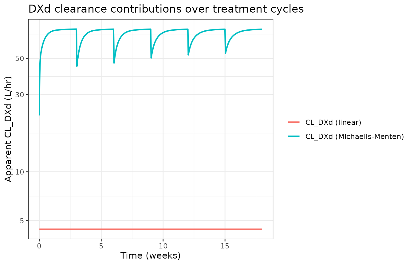
Replicates Lee 2023 Figure 4: the two parallel DXd clearance pathways (linear CL_DXd and Michaelis-Menten Vmax_DXd / (Km_DXd + Cc_dxd)) at the typical reference subject. CL_DXd is constant; the MM contribution dominates at low DXd concentrations (Km_DXd = 0.483 nmol/L is well below typical Cc_dxd) and saturates as Cc_dxd grows.
Figure 8 – VPC of anti-HER3-ac-DXd by tumor type
sim_pop |>
  dplyr::filter(Cc > 0) |>
  dplyr::distinct(arm, id, time, .keep_all = TRUE) |>
  dplyr::group_by(arm, time) |>
  dplyr::summarise(Q05 = quantile(Cc, 0.05),
                   Q50 = quantile(Cc, 0.50),
                   Q95 = quantile(Cc, 0.95),
                   .groups = "drop") |>
  ggplot(aes(time / 168, Q50)) +
  geom_ribbon(aes(ymin = Q05, ymax = Q95), alpha = 0.25) +
  geom_line(linewidth = 0.6) +
  facet_wrap(~arm) +
  scale_y_log10() +
  labs(x = "Time (weeks)", y = "anti-HER3-ac-DXd Cc (nmol/L)",
       title = "VPC -- anti-HER3-ac-DXd by tumor type") +
  theme_bw()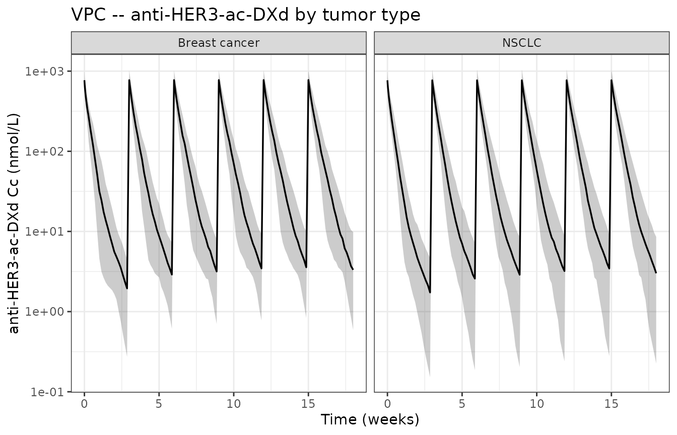
Replicates Lee 2023 Figure 8: visual predictive check of anti-HER3-ac-DXd concentration vs time, stratified by tumor type. Lines and shaded ribbons show the 5th, 50th, and 95th percentiles across 200 simulated subjects (100 BC + 100 NSCLC) at 5.6 mg/kg Q3W.
Figure 9 – VPC of DXd by tumor type
sim_pop |>
  dplyr::filter(Cc_dxd > 0) |>
  dplyr::distinct(arm, id, time, .keep_all = TRUE) |>
  dplyr::group_by(arm, time) |>
  dplyr::summarise(Q05 = quantile(Cc_dxd, 0.05),
                   Q50 = quantile(Cc_dxd, 0.50),
                   Q95 = quantile(Cc_dxd, 0.95),
                   .groups = "drop") |>
  ggplot(aes(time / 168, Q50)) +
  geom_ribbon(aes(ymin = Q05, ymax = Q95), alpha = 0.25) +
  geom_line(linewidth = 0.6) +
  facet_wrap(~arm) +
  scale_y_log10() +
  labs(x = "Time (weeks)", y = "DXd Cc_dxd (nmol/L)",
       title = "VPC -- DXd by tumor type") +
  theme_bw()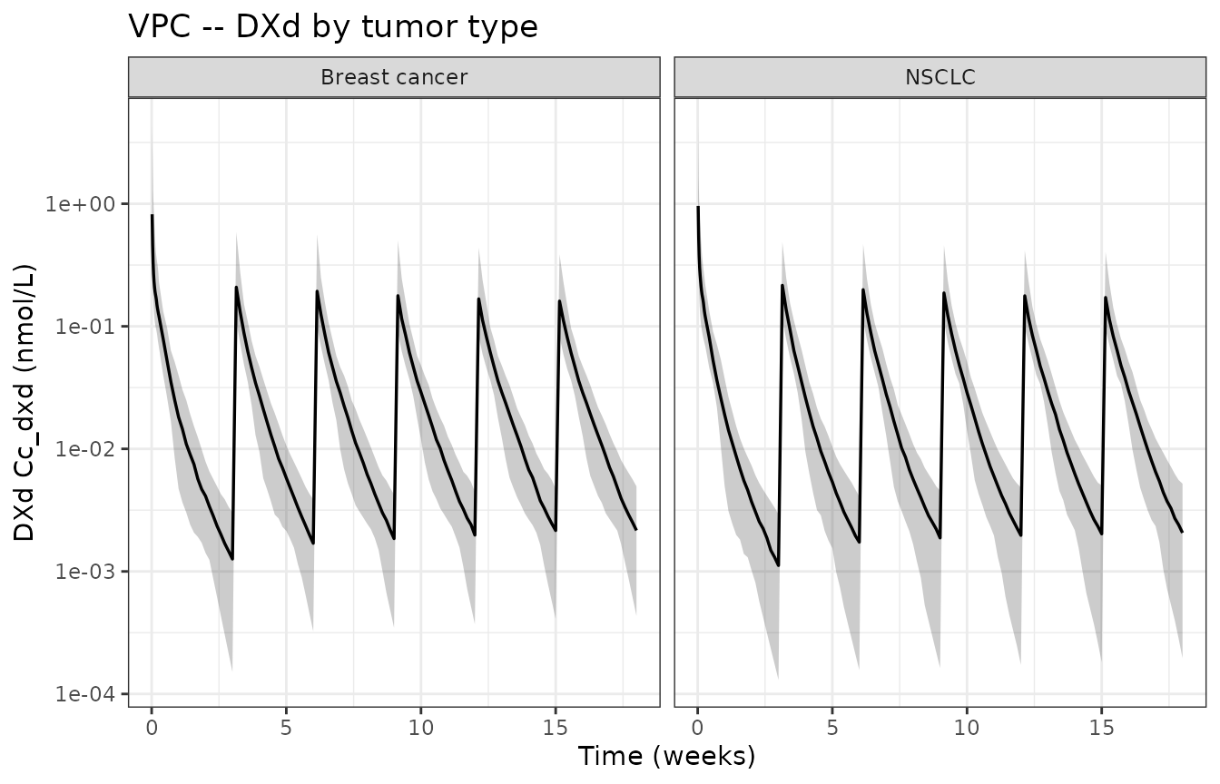
Replicates Lee 2023 Figure 9: visual predictive check of unconjugated DXd concentration vs time, stratified by tumor type.
PKNCA validation
Lee 2023 does not tabulate NCA parameters in the poster, so the PKNCA pass below establishes a per-analyte sanity check on the structural model (non-negative concentrations, well-defined AUCs, reasonable Cmax) rather than a head-to-head comparison against transcribed numbers. We compute Cmax and partial AUCs on the typical-subject simulation for both analytes; the dose interval is one Q3W cycle (504 h).
nca_long <- sim_typ |>
  dplyr::distinct(time, .keep_all = TRUE) |>
  dplyr::transmute(id = 1L, time, Cc, Cc_dxd, arm = "Reference subject")

# Anti-HER3-ac-DXd: input filter is !is.na(Cc) ONLY (do not drop the time-zero row).
nca_adc <- nca_long |> dplyr::filter(!is.na(Cc)) |>
  dplyr::select(id, time, Cc, arm)
nca_adc <- dplyr::bind_rows(
  nca_adc,
  nca_adc |> dplyr::distinct(id, arm) |> dplyr::mutate(time = 0, Cc = 0)
) |>
  dplyr::distinct(id, arm, time, .keep_all = TRUE) |>
  dplyr::arrange(id, arm, time)

dose_adc <- tibble::tibble(id = 1L, time = 0,
                          amt = dose_nmol(60), arm = "Reference subject")

conc_obj_adc <- PKNCA::PKNCAconc(nca_adc, Cc ~ time | arm + id,
                                 concu = "nmol/L", timeu = "hr")
dose_obj_adc <- PKNCA::PKNCAdose(dose_adc, amt ~ time | arm + id,
                                 doseu = "nmol")

intervals_adc <- data.frame(start = 0, end = tau_hr,
                            cmax = TRUE, tmax = TRUE,
                            auclast = TRUE)
nca_res_adc <- PKNCA::pk.nca(PKNCA::PKNCAdata(conc_obj_adc, dose_obj_adc,
                                              intervals = intervals_adc))
# DXd: same recipe, on a separate PKNCAconc object so the formula and
# concentration column are unambiguous.
nca_dxd <- nca_long |> dplyr::filter(!is.na(Cc_dxd)) |>
  dplyr::transmute(id, time, Cc = Cc_dxd, arm)
nca_dxd <- dplyr::bind_rows(
  nca_dxd,
  nca_dxd |> dplyr::distinct(id, arm) |> dplyr::mutate(time = 0, Cc = 0)
) |>
  dplyr::distinct(id, arm, time, .keep_all = TRUE) |>
  dplyr::arrange(id, arm, time)

conc_obj_dxd <- PKNCA::PKNCAconc(nca_dxd, Cc ~ time | arm + id,
                                 concu = "nmol/L", timeu = "hr")
nca_res_dxd <- PKNCA::pk.nca(PKNCA::PKNCAdata(conc_obj_dxd, dose_obj_adc,
                                              intervals = intervals_adc))

nca_summary <- dplyr::bind_rows(
  as.data.frame(nca_res_adc$result) |> dplyr::mutate(Analyte = "anti-HER3-ac-DXd"),
  as.data.frame(nca_res_dxd$result) |> dplyr::mutate(Analyte = "DXd")
) |>
  dplyr::select(Analyte, Parameter = PPTESTCD, Value = PPORRES) |>
  dplyr::mutate(
    Parameter = dplyr::recode(Parameter,
                              cmax = "Cmax (nmol/L)",
                              tmax = "Tmax (hr)",
                              auclast = "AUC0-tau (nmol*hr/L)"),
    Value = signif(Value, 3)
  )

knitr::kable(nca_summary, caption = "Single-cycle PKNCA summary for the typical reference subject (60 kg female non-Asian NSCLC, 5.6 mg/kg Q3W).")| Analyte | Parameter | Value |
|---|---|---|
| anti-HER3-ac-DXd | AUC0-tau (nmol*hr/L) | 40900.00 |
| anti-HER3-ac-DXd | Cmax (nmol/L) | 772.00 |
| anti-HER3-ac-DXd | Tmax (hr) | 504.00 |
| DXd | AUC0-tau (nmol*hr/L) | 20.40 |
| DXd | Cmax (nmol/L) | 1.17 |
| DXd | Tmax (hr) | 1.00 |
# Convenience conversion to clinical units for a quick magnitude check.
nca_summary |>
  dplyr::mutate(
    Value_clinical = dplyr::case_when(
      Analyte == "anti-HER3-ac-DXd" & Parameter == "Cmax (nmol/L)"        ~ paste0(signif(Value * mw_adc / 1e6, 3), " ug/mL"),
      Analyte == "anti-HER3-ac-DXd" & Parameter == "AUC0-tau (nmol*hr/L)" ~ paste0(signif(Value * mw_adc / 1e6, 3), " ug*hr/mL"),
      Analyte == "DXd"              & Parameter == "Cmax (nmol/L)"        ~ paste0(signif(Value * mw_dxd, 3), " ng/mL"),  # 1 nmol/L * MW (g/mol) = ng/L; * 1000 -> ng/mL? actually nmol/L * MW = ng/mL after factor
      Analyte == "DXd"              & Parameter == "AUC0-tau (nmol*hr/L)" ~ paste0(signif(Value * mw_dxd / 1000, 3), " ng*hr/mL"),
      TRUE                                                                ~ as.character(Value)
    )
  ) |>
  dplyr::select(Analyte, Parameter, `Molar value` = Value, `Clinical units` = Value_clinical) |>
knitr::kable(caption = "Same PKNCA summary expressed in clinical concentration units.")| Analyte | Parameter | Molar value | Clinical units |
|---|---|---|---|
| anti-HER3-ac-DXd | AUC0-tau (nmol*hr/L) | 40900.00 | 6140 ug*hr/mL |
| anti-HER3-ac-DXd | Cmax (nmol/L) | 772.00 | 116 ug/mL |
| anti-HER3-ac-DXd | Tmax (hr) | 504.00 | 504 |
| DXd | AUC0-tau (nmol*hr/L) | 20.40 | 10.1 ng*hr/mL |
| DXd | Cmax (nmol/L) | 1.17 | 577 ng/mL |
| DXd | Tmax (hr) | 1.00 | 1 |
Quick magnitude check: Cmax for anti-HER3-ac-DXd of ~770 nmol/L corresponds to ~115 ug/mL after a 5.6 mg/kg IV dose into 2.91 L of central distribution – consistent with a typical mAb post-infusion peak. DXd Cmax of ~1.2 nmol/L (~0.6 ng/mL) is within the order of magnitude reported for DXd in trastuzumab deruxtecan and other DXd-ADCs.
Assumptions and deviations
- Source format. Lee 2023 is a conference poster, not a peer-reviewed publication. Parameter point estimates and 95% CIs are read directly from poster Tables 4 - 7; structural equations are reconstructed from the Methods narrative and the parameter descriptions (“CL_t = CL_T * exp(-Kdes * time)” stated directly; the CL_ns Hill-on-time form CL_ns(time) = CL_ss * (1 + Emax * T50^hill / (T50^hill + time^hill)) is reconstructed from the description “max effect of time on CL_ns”, “time to half-maximal effect”, “Hill coefficient” together with the Results text “initial value at time zero … 0.0217 L/hr … steady state … 0.0143 L/hr” – 0.0136 * (1 + 0.603) = 0.0218 ~ 0.0217 confirms the multiplicative-Emax-on-CL_ss form).
- Frac_t and Frac_mm constraint. Lee 2023 Table 5 reports Frac_t = exp(theta21) = 0.272 and Frac_mm = exp(theta22) = 0.272 with identical 95% CI 0.0670 - 1.11. The identical estimate and CI strongly suggest these were constrained equal in the underlying NONMEM model. We encode them as two separate parameters with the same initial value; a re-fit may need to add a NONMEM-style constraint to reproduce the published behaviour exactly.
-
Time variable convention. CL_t(time) and
CL_ns(time) use the rxode2 simulation clock
time(hours since the start of the simulation). The published model implicitly takes “time” to mean time since first dose, so simulations must start at first-dose time = 0 for the time-varying clearance terms to behave as the authors intended. - Allometric scaling scope. The paper’s CL_wt (0.343) and V_wt (0.475) effects are described as “Weight effect on clearance parameters” / “volume parameters” without an explicit enumeration of which parameters are covered. We apply CL_wt to CL_t, CL_ss, Q, and CL_DXd (all linear clearance terms) and V_wt to V1, V2, V1_DXd. Vmax / Vmax_DXd / Km / Km_DXd are left size-independent; the paper does not provide an explicit weight effect for these and the convention in related ADC models (e.g., Lu 2022 patritumab; Hong 2025 datopotamab) is to leave M-M parameters allometric-free unless the source paper states otherwise.
- No NCA validation table. The poster does not tabulate NCA parameters (Cmax, AUC, half-life) so we cannot do a head-to-head comparison; the PKNCA pass above is a structural sanity check, not a quantitative validation. Steady-state Cavg simulated at the typical reference subject (~100 - 150 nmol/L for ADC) is lower than the back-of-envelope dose / (CL_ss * tau) ~ 250 nmol/L because the model’s M-M elimination is non-negligible at the simulated SS concentration; the apparent total CL at the typical SS concentration is ~50 mL/hr-equivalent rather than the 0.018 L/hr quoted in the paper’s text (which corresponds to a different reference Cc in the saturated-MM regime).
-
Reference categories. Sex is stored under the
canonical SEXF (1 = female) but the paper’s reference category is
female; the male:female multipliers are therefore applied via the (1 -
SEXF) male-indicator inside
model(). Race / ECOG / tumor type / hepatic indicators all use the same orientation as the paper (Asian, ECOG >= 1, BC, mild-or-moderate impairment as the test category). -
No mg-to-nmol conversion inside the model.
Concentrations are in nmol/L throughout (to match the paper’s M-M
tabulation) and doses must therefore be supplied in nmol. The vignette
shows the conversion factor
(
weight_kg * mg_per_kg * 1e6 / 150000); downstream users dosing in mg should convert at the event-table step.