Inhaled fluticasone furoate and vilanterol in COPD (Siederer 2016) • nlmixr2lib

Model and source

Citation: Siederer S, Allen A, Yang S. Population Pharmacokinetics of Inhaled Fluticasone Furoate and Vilanterol in Subjects with Chronic Obstructive Pulmonary Disease. Eur J Drug Metab Pharmacokinet. 2016;41(6):743-758. doi:10.1007/s13318-015-0303-4
Article (open access): https://doi.org/10.1007/s13318-015-0303-4
Online Resource (Tables S1-S2, Figs. S1-S2): supplementary PDF 13318_2015_303_MOESM1_ESM.pdf attached to the article record (PMC5119845).

Fluticasone furoate (FF, an inhaled corticosteroid) and vilanterol (VI, a long-acting beta2-agonist) are co-formulated in a single dry-powder inhaler (ELLIPTA) for maintenance treatment of COPD. Earlier characterisations of both molecules rested on small non-compartmental studies whose profiles were heavily censored, because inhaled systemic exposure sits close to the assay limit of quantification. Siederer 2016 pools concentration-time data from three Phase III COPD trials, one Phase II COPD trial and one intensively-sampled Phase I healthy-volunteer study, and fits it with the NONMEM M3 likelihood so that the 39% (FF) and 30% (VI) of records below the limit of quantification contribute as censored observations rather than being discarded.

The paper contains two independent models, stated explicitly in Sect. 2.3: “The FF and VI concentration-time data were modeled independently.” They share neither parameters nor a likelihood, so they are extracted as two model files:

ff <- rxode2::rxode(readModelDb("Siederer_2016_fluticasoneFuroate"))
#> ℹ parameter labels from comments will be replaced by 'label()'
vi <- rxode2::rxode(readModelDb("Siederer_2016_vilanterol"))
#> ℹ parameter labels from comments will be replaced by 'label()'

	Fluticasone furoate	Vilanterol
Structure	2-compartment (ADVAN4 TRANS4)	3-compartment (ADVAN11 TRANS4)
Absorption	first-order, `ka`	zero-order, duration `D1`
Analysis dataset	1307 subjects, 11,789 obs, 39% BLQ	1167 subjects, 10,807 obs, 30% BLQ
Studies	4 (Phase II study excluded)	5
Covariates retained	race on CL/F	age + weight + study on CL/F; age + sex + smoking + study on V1/F
Residual error	additive on the linear concentration scale	additive on the log concentration scale

Units

Both model files declare dosing = "ug" and volumes in L, so Cc is in ug/L, i.e. ng/mL. Siederer 2016 reports every concentration and exposure in pg/mL and pg*h/mL. The conversion factor is therefore 1000, applied explicitly wherever simulated output is compared with the paper:

NG_PER_ML_TO_PG_PER_ML <- 1000

No scale factor is buried inside either model, so dose, volume and clearance stay mutually consistent and the mass-balance identity below can be used as a gate.

Population

Demographics are Online Resource Table S2; study designs are Table S1.

pop <- rxode2::rxode(readModelDb("Siederer_2016_vilanterol"))$meta$population
#> ℹ parameter labels from comments will be replaced by 'label()'
tibble::tibble(
  Field = c(
    "Species", "N (FF analysis)", "N (VI analysis)", "Median age",
    "Age range", "Mean weight", "Weight range", "Female", "White/Caucasian",
    "COPD", "Mean % predicted FEV1 (COPD)"
  ),
  Value = c(
    "human", "1307", "1167", "61.0 years", "18-85 years", "75.3-75.7 kg",
    "34.6-174.6 kg", "67-68%", "82%", "94%", "48.1-48.8%"
  )
) |>
  knitr::kable(caption = "Online Resource Table S2, both analysis datasets.")

Online Resource Table S2, both analysis datasets.
Field	Value
Species	human
N (FF analysis)	1307
N (VI analysis)	1167
Median age	61.0 years
Age range	18-85 years
Mean weight	75.3-75.7 kg
Weight range	34.6-174.6 kg
Female	67-68%
White/Caucasian	82%
COPD	94%
Mean % predicted FEV1 (COPD)	48.1-48.8%

The five contributing studies (Online Resource Table S1):

tibble::tibble(
  Study = c("1", "2", "3", "4", "5"),
  Protocol = c("HZC112206", "HZC112207", "HZC110946", "HZC111348", "HZA102936"),
  Phase = c("III", "III", "III", "II", "I"),
  Population = c("COPD", "COPD", "COPD", "COPD", "Healthy"),
  `FF/VI doses (ug)` = c(
    "50/25, 100/25", "100/25, 200/25", "50/25, 100/25, 200/25",
    "400/25", "200/25, 800/100"
  ),
  `In FF analysis` = c("yes", "yes", "yes", "no (0-4 h data only)", "yes"),
  `In VI analysis` = c("yes", "yes", "yes", "yes", "yes")
) |>
  knitr::kable(caption = "Online Resource Table S1.")

Online Resource Table S1.
Study	Protocol	Phase	Population	FF/VI doses (ug)	In FF analysis	In VI analysis
1	HZC112206	III	COPD	50/25, 100/25	yes	yes
2	HZC112207	III	COPD	100/25, 200/25	yes	yes
3	HZC110946	III	COPD	50/25, 100/25, 200/25	yes	yes
4	HZC111348	II	COPD	400/25	no (0-4 h data only)	yes
5	HZA102936	I	Healthy	200/25, 800/100	yes	yes

Source trace

Every ini() value, with the exact location it was read from. Both tables in the paper print each THETA twice, as a log-scale “Ln estimate” and as its exponential “Estimate”; the model files encode log(<untransformed estimate>) because that column carries more significant figures.

tibble::tribble(
  ~Parameter, ~Value, ~Source,
  "lka", "log(0.0523)", "Table 1 row 'ka (h-1)' (Ln estimate -2.95)",
  "lcl", "log(230)", "Table 1 row 'CL/F (L/h)'; Sect. 3.1.2 typical value",
  "lvc", "fixed(log(1.36))", "Table 1 row 'V2/F (L)' = 1.36 FIXED; Sect. 3.1.2",
  "lq", "log(268)", "Table 1 row 'Q/F (L/h)'",
  "lvp", "log(111)", "Table 1 row 'V3/F (L)'",
  "e_race_asian_east_se_cl", "-0.211", "Table 1 row 'RACE1 = 2 on CL/F' Ln estimate",
  "e_race_black_cl", "0.0602", "Table 1 row 'RACE1 = 3 on CL/F' Ln estimate",
  "e_race_asian_central_arabic_amind_oth_cl", "-0.265", "Table 1 row 'RACE1 = 4 on CL/F' Ln estimate",
  "race covariate equation", "Ln(theta) = theta_1 + COV", "Sect. 3.1.2 Eq. (a)",
  "etalcl", "fixed(0)", "Sect. 3.1.2 (IIV declared, magnitude not reported)",
  "addSd", "fixed(0)", "Sect. 3.1.2 additive error; magnitude not reported"
) |>
  knitr::kable(caption = "Fluticasone furoate model (Siederer 2016 Table 1).")

Fluticasone furoate model (Siederer 2016 Table 1).
Parameter	Value	Source
lka	log(0.0523)	Table 1 row ‘ka (h-1)’ (Ln estimate -2.95)
lcl	log(230)	Table 1 row ‘CL/F (L/h)’; Sect. 3.1.2 typical value
lvc	fixed(log(1.36))	Table 1 row ‘V2/F (L)’ = 1.36 FIXED; Sect. 3.1.2
lq	log(268)	Table 1 row ‘Q/F (L/h)’
lvp	log(111)	Table 1 row ‘V3/F (L)’
e_race_asian_east_se_cl	-0.211	Table 1 row ‘RACE1 = 2 on CL/F’ Ln estimate
e_race_black_cl	0.0602	Table 1 row ‘RACE1 = 3 on CL/F’ Ln estimate
e_race_asian_central_arabic_amind_oth_cl	-0.265	Table 1 row ‘RACE1 = 4 on CL/F’ Ln estimate
race covariate equation	Ln(theta) = theta_1 + COV	Sect. 3.1.2 Eq. (a)
etalcl	fixed(0)	Sect. 3.1.2 (IIV declared, magnitude not reported)
addSd	fixed(0)	Sect. 3.1.2 additive error; magnitude not reported

tibble::tribble(
  ~Parameter, ~Value, ~Source,
  "lcl_copd", "log(94.6)", "Table 2 row 'CL/F, COPD (L/h)'; Sect. 3.2.2 typical value",
  "lcl_hvt", "log(135.6)", "Table 2 row 'CL/F, HVT (L/h)'",
  "lvc_copd", "log(639.0)", "Table 2 row 'V1/F, COPD (L)'; Sect. 3.2.2 typical value",
  "lvc_hvt", "log(159.2)", "Table 2 row 'V1/F, HVT (L)'",
  "lvp_copd", "log(177.7)", "Table 2 row 'V2/F, COPD (L)'",
  "lvp_hvt", "log(507.8)", "Table 2 row 'V2/F, HVT (L)'",
  "lq", "log(242.3)", "Table 2 row 'Q2/F (L/h)'",
  "lq2", "log(141.2)", "Table 2 row 'Q3/F (L/h)'",
  "lvp2", "log(2100.6)", "Table 2 row 'V3/F' (header unit misprinted as L/h)",
  "ld1", "log(0.098)", "Table 2 row 'D1 (h)'",
  "e_age_cl", "-0.433", "Table 2 row 'Age on CL/F, COPD' Ln estimate",
  "e_wt_cl", "0.421", "Table 2 row 'Wt on CL/F, COPD' Ln estimate",
  "e_age_vc", "-0.499", "Table 2 row 'Age on V1/F, COPD' Ln estimate",
  "e_sexf_vc", "-0.128", "Table 2 row 'Sex on V1/F, COPD' Ln estimate",
  "e_smoke_vc", "0.295", "Table 2 row 'Smoking on V1/F, COPD' Ln estimate",
  "e_study_hzc111348_cl", "-0.465", "Table 2 row 'Study 4 on CL/F, COPD' Ln estimate",
  "e_study_hzc110946_vc", "-0.358", "Table 2 row 'Study 3 on V1/F, COPD' Ln estimate",
  "e_study_hzc111348_vc", "-1.24", "Table 2 row 'Study 4 on V1/F, COPD' Ln estimate",
  "categorical covariate equation", "Ln CL = theta_1 + theta_COV x (cov - 1)", "Sect. 3.2.2 Eq. (b)",
  "continuous covariate equation", "power model, see Errata", "Sect. 3.2.2 Eq. (c), as corrected",
  "etalcl, etalvp2", "fixed(0)", "Sect. 2.5 / Sect. 3.2.2 (IIV declared, magnitudes not reported)",
  "expSd", "fixed(0)", "Sect. 3.2.2 additive error on the log scale; magnitude not reported"
) |>
  knitr::kable(caption = "Vilanterol model (Siederer 2016 Table 2).")

Vilanterol model (Siederer 2016 Table 2).
Parameter	Value	Source
lcl_copd	log(94.6)	Table 2 row ‘CL/F, COPD (L/h)’; Sect. 3.2.2 typical value
lcl_hvt	log(135.6)	Table 2 row ‘CL/F, HVT (L/h)’
lvc_copd	log(639.0)	Table 2 row ‘V1/F, COPD (L)’; Sect. 3.2.2 typical value
lvc_hvt	log(159.2)	Table 2 row ‘V1/F, HVT (L)’
lvp_copd	log(177.7)	Table 2 row ‘V2/F, COPD (L)’
lvp_hvt	log(507.8)	Table 2 row ‘V2/F, HVT (L)’
lq	log(242.3)	Table 2 row ‘Q2/F (L/h)’
lq2	log(141.2)	Table 2 row ‘Q3/F (L/h)’
lvp2	log(2100.6)	Table 2 row ‘V3/F’ (header unit misprinted as L/h)
ld1	log(0.098)	Table 2 row ‘D1 (h)’
e_age_cl	-0.433	Table 2 row ‘Age on CL/F, COPD’ Ln estimate
e_wt_cl	0.421	Table 2 row ‘Wt on CL/F, COPD’ Ln estimate
e_age_vc	-0.499	Table 2 row ‘Age on V1/F, COPD’ Ln estimate
e_sexf_vc	-0.128	Table 2 row ‘Sex on V1/F, COPD’ Ln estimate
e_smoke_vc	0.295	Table 2 row ‘Smoking on V1/F, COPD’ Ln estimate
e_study_hzc111348_cl	-0.465	Table 2 row ‘Study 4 on CL/F, COPD’ Ln estimate
e_study_hzc110946_vc	-0.358	Table 2 row ‘Study 3 on V1/F, COPD’ Ln estimate
e_study_hzc111348_vc	-1.24	Table 2 row ‘Study 4 on V1/F, COPD’ Ln estimate
categorical covariate equation	Ln CL = theta_1 + theta_COV x (cov - 1)	Sect. 3.2.2 Eq. (b)
continuous covariate equation	power model, see Errata	Sect. 3.2.2 Eq. (c), as corrected
etalcl, etalvp2	fixed(0)	Sect. 2.5 / Sect. 3.2.2 (IIV declared, magnitudes not reported)
expSd	fixed(0)	Sect. 3.2.2 additive error on the log scale; magnitude not reported

Fluticasone furoate

Typical clearance by race category

Sect. 3.1.2 quotes the typical CL/F for each of the four race groupings. Because FF carries no continuous covariate and no estimable IIV, these are exact predictions of the model, so they can be checked to the paper’s printed precision.

ff_race <- tibble::tibble(
  race_label = c(
    "1: White/Caucasian",
    "2: East Asian / Japanese / South East Asian",
    "3: African American",
    "4: Central Asian / White-Arabic / Am. Indian / other"
  ),
  RACE_ASIAN_EAST_SE = c(0, 1, 0, 0),
  RACE_BLACK = c(0, 0, 1, 0),
  RACE_ASIAN_CENTRAL_ARABIC_AMIND_OTH = c(0, 0, 0, 1),
  paper_cl = c(230, 186, 244, 176)
) |>
  mutate(
    model_cl = exp(
      log(230) - 0.211 * RACE_ASIAN_EAST_SE + 0.0602 * RACE_BLACK -
        0.265 * RACE_ASIAN_CENTRAL_ARABIC_AMIND_OTH
    )
  )

ff_race |>
  select(race_label, paper_cl, model_cl) |>
  rename(
    "Race grouping (RACE1)" = race_label,
    "Sect. 3.1.2 CL/F (L/h)" = paper_cl,
    "Model CL/F (L/h)" = model_cl
  ) |>
  knitr::kable(digits = 1)

Race grouping (RACE1)	Sect. 3.1.2 CL/F (L/h)	Model CL/F (L/h)
1: White/Caucasian	230	230.0
2: East Asian / Japanese / South East Asian	186	186.2
3: African American	244	244.3
4: Central Asian / White-Arabic / Am. Indian / other	176	176.5


# Strict: the model must round to each printed value.
stopifnot(all(round(ff_race$model_cl) == ff_race$paper_cl))

Steady-state simulation

Once-daily inhalation. ss = 1 puts the system at steady state directly rather than integrating a 30-dose train.

ff_doses <- c(50, 100, 200)

ff_events <-
  tidyr::expand_grid(
    dose = ff_doses,
    race_idx = seq_len(nrow(ff_race))
  ) |>
  mutate(id = dplyr::row_number()) |>
  rowwise() |>
  group_split() |>
  lapply(function(g) {
    dose_row <- data.frame(
      id = g$id, time = 0, amt = g$dose, evid = 1, cmt = "depot",
      ii = 24, ss = 1
    )
    obs_row <- data.frame(
      id = g$id, time = seq(0, 24, by = 0.02), amt = NA_real_, evid = 0,
      cmt = "central", ii = 0, ss = 0
    )
    out <- dplyr::bind_rows(dose_row, obs_row)
    out$dose <- g$dose
    out$race_idx <- g$race_idx
    out
  }) |>
  dplyr::bind_rows() |>
  left_join(
    ff_race |> mutate(race_idx = dplyr::row_number()) |>
      select(
        race_idx, race_label, RACE_ASIAN_EAST_SE, RACE_BLACK,
        RACE_ASIAN_CENTRAL_ARABIC_AMIND_OTH
      ),
    by = "race_idx"
  ) |>
  arrange(id, time, dplyr::desc(evid))

ff_sim <- rxode2::rxSolve(
  ff, ff_events,
  keep = c("dose", "race_label"),
  returnType = "data.frame"
)
#> ℹ omega/sigma items treated as zero: 'etalcl'
#> Warning: multi-subject simulation without without 'omega'

ff_sim |>
  filter(!is.na(Cc)) |>
  mutate(Cc_pg = Cc * NG_PER_ML_TO_PG_PER_ML) |>
  ggplot(aes(time, Cc_pg, colour = race_label)) +
  geom_line() +
  facet_wrap(~ paste0(dose, " ug once daily")) +
  labs(
    x = "Time after dose (h)", y = "FF concentration (pg/mL)",
    colour = "RACE1 grouping"
  ) +
  theme_bw() +
  theme(legend.position = "bottom", legend.direction = "vertical")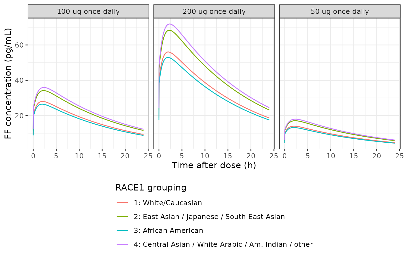

Steady-state fluticasone furoate plasma concentration over one 24 h dosing interval, by nominal dose and race grouping. Compare the shape with Fig. 2 of Siederer 2016 (VPC by dose regimen).

The profile is strikingly flat: the estimated ka of 0.0523 /h corresponds to an absorption half-life of 13.3 h against a disposition half-life well under an hour, so inhaled FF is deeply flip-flop and the terminal slope is the absorption rate. That is the pharmacology the model encodes, and it is why trough concentrations in the Phase III trials were frequently quantifiable despite a very low peak.

Mass-balance gate

At steady state, AUC over the dosing interval must equal dose / CL exactly. This gate uses no published number, so it cannot be satisfied by a transcription error in either direction – it tests the ODE system, the compartment mapping and the unit declaration together.

ff_auc <- ff_sim |>
  filter(!is.na(Cc)) |>
  group_by(id, dose, race_label) |>
  summarise(
    auc_tau = sum(diff(time) * (head(Cc, -1) + tail(Cc, -1)) / 2),
    .groups = "drop"
  ) |>
  left_join(
    ff_race |> select(race_label, model_cl), by = "race_label"
  ) |>
  mutate(
    dose_over_cl = dose / model_cl,
    rel_err = (auc_tau - dose_over_cl) / dose_over_cl
  )

# The residual is pure trapezoidal quadrature error on the observation grid,
# and converges as O(h^2): the relative error is 1.16e-3 at a 0.1 h grid,
# 5.41e-4 at 0.05 h, 1.76e-4 at 0.02 h (used here) and 6.12e-5 at 0.01 h.
# A structural fault -- wrong compartment mapping, wrong unit declaration,
# a mis-transcribed clearance -- moves this by tens of percent, so 1e-3
# is a strict gate at this grid density and not a tuned tolerance.
stopifnot(max(abs(ff_auc$rel_err)) < 1e-3)
sprintf(
  "AUC(0-tau) matches dose/CL for all %d profiles; max relative error %.2e",
  nrow(ff_auc), max(abs(ff_auc$rel_err))
)
#> [1] "AUC(0-tau) matches dose/CL for all 12 profiles; max relative error 1.84e-04"

Non-compartmental analysis

The race grouping is carried into the PKNCA formula alongside dose, so each of the twelve dose x race profiles gets its own NCA rather than being collapsed. That matters for the comparison below: Table 3’s “FF dose” rows pool the whole dataset, which is 82% White/Caucasian, so the correct comparator for them is the White/Caucasian profile – not a median over four equally-weighted race arms, which would sit about 12% high.

ff_conc <- ff_sim |>
  filter(!is.na(Cc)) |>
  transmute(
    id = factor(id), time, treatment = paste0(dose, " ug"),
    race_label,
    Cc = Cc * NG_PER_ML_TO_PG_PER_ML
  )

ff_dose_df <- ff_events |>
  filter(evid == 1) |>
  transmute(
    id = factor(id), time, amt = dose, treatment = paste0(dose, " ug"),
    race_label
  )

ff_conc_obj <- PKNCA::PKNCAconc(
  ff_conc, Cc ~ time | treatment + race_label + id,
  concu = "pg/mL", timeu = "h"
)
ff_dose_obj <- PKNCA::PKNCAdose(
  ff_dose_df, amt ~ time | treatment + race_label + id,
  doseu = "ug"
)

ff_intervals <- data.frame(
  start = 0, end = 24,
  cmax = TRUE, tmax = TRUE, cmin = TRUE, auclast = TRUE, cav = TRUE
)

ff_nca <- PKNCA::pk.nca(
  PKNCA::PKNCAdata(ff_conc_obj, ff_dose_obj, intervals = ff_intervals)
)

# White/Caucasian reference profiles only, for comparison with Table 3.
ff_white <- as.data.frame(ff_nca$result) |>
  filter(race_label == ff_race$race_label[1]) |>
  select(treatment, PPTESTCD, PPORRES)

Comparison against the published race effect

Siederer 2016 Table 3 reports model-predicted steady-state AUC0-24 stratified by dose and race grouping. The ratio of each race group’s AUC to the White/Caucasian AUC is a scale-free test of the covariate coefficients, and it is the comparison the model can be held to: AUC is inversely proportional to CL/F, so the predicted ratio is simply exp(-coefficient).

table3_auc <- tibble::tribble(
  ~dose, ~race1, ~race2, ~race3, ~race4, ~n2, ~n3, ~n4,
  50, 79.05, 102.77, 81.19, 99.25, 37L, 16L, 4L,
  100, 176.04, 223.04, 128.25, 202.34, 111L, 13L, 9L,
  200, 319.68, 394.61, 245.42, 352.68, 20L, 17L, 3L
)

ratio_tbl <- table3_auc |>
  transmute(
    Dose = paste0(dose, " ug"),
    `RACE1 = 2` = race2 / race1,
    `RACE1 = 3` = race3 / race1,
    `RACE1 = 4` = race4 / race1
  ) |>
  tidyr::pivot_longer(-Dose, names_to = "Grouping", values_to = "Table 3 ratio") |>
  mutate(
    `Model ratio` = dplyr::case_when(
      Grouping == "RACE1 = 2" ~ exp(0.211),
      Grouping == "RACE1 = 3" ~ exp(-0.0602),
      Grouping == "RACE1 = 4" ~ exp(0.265)
    ),
    `% diff` = 100 * (`Table 3 ratio` - `Model ratio`) / `Model ratio`
  )

ratio_tbl |>
  knitr::kable(
    digits = c(0, 0, 3, 3, 1),
    caption = paste(
      "AUC0-24 ratio versus White/Caucasian. The model ratio is exp(-coefficient)",
      "and does not depend on dose."
    )
  )

AUC0-24 ratio versus White/Caucasian. The model ratio is exp(-coefficient) and does not depend on dose.
Dose	Grouping	Table 3 ratio	Model ratio	% diff
50 ug	RACE1 = 2	1.300	1.235	5.3
50 ug	RACE1 = 3	1.027	0.942	9.1
50 ug	RACE1 = 4	1.256	1.303	-3.7
100 ug	RACE1 = 2	1.267	1.235	2.6
100 ug	RACE1 = 3	0.729	0.942	-22.6
100 ug	RACE1 = 4	1.149	1.303	-11.8
200 ug	RACE1 = 2	1.234	1.235	0.0
200 ug	RACE1 = 3	0.768	0.942	-18.5
200 ug	RACE1 = 4	1.103	1.303	-15.4

RACE1 = 2 is the only race coefficient the paper estimates well (%RSE 28.5, N = 111 at the 100 ug dose, and the 95% CI excludes 1). Its Table 3 ratio must therefore match the model closely at every dose:

race2 <- ratio_tbl |> filter(Grouping == "RACE1 = 2")
stopifnot(
  # Structural: a mis-signed or mis-scaled race coefficient blows this instantly.
  max(abs(race2$`% diff`)) < 6
)
sprintf(
  "RACE1 = 2 AUC ratio reproduced at all three doses; max |%% diff| = %.1f%%",
  max(abs(race2$`% diff`))
)
#> [1] "RACE1 = 2 AUC ratio reproduced at all three doses; max |% diff| = 5.3%"

RACE1 = 3 (%RSE 199, 95% CI spans 1, N = 13-17) and RACE1 = 4 (%RSE 50.6, N = 3-9) scatter widely, which is exactly what Sect. 3.1.2 warns about: “the fixed-effect parameter RACE1 = 3 was estimated with less precision (%RSE 199 %) and should thus be interpreted with caution”. Table 3’s values are summaries of post hoc individual estimates in cells holding as few as three subjects, so they are not held to a tolerance here.

Comparison against published absolute exposures

table3_abs <- tibble::tribble(
  ~treatment, ~cmax, ~auclast,
  "50 ug", 7.52, 82.92,
  "100 ug", 11.73, 181.82,
  "200 ug", 21.62, 319.69
)

ff_cmp <- nlmixr2lib::ncaComparisonTable(
  simulated = ff_white,
  reference = table3_abs,
  by = "treatment",
  params = c("cmax", "auclast"),
  units = c(cmax = "pg/mL", auclast = "pg*h/mL")
)
knitr::kable(ff_cmp, digits = 1)

NCA parameter	treatment	Reference	Simulated	% diff
Cmax (pg/mL)	50 ug	7.52	14	+86.3%*
Cmax (pg/mL)	100 ug	11.7	28	+138.8%*
Cmax (pg/mL)	200 ug	21.6	56	+159.1%*
AUClast (pg*h/mL)	50 ug	82.9	217	+162.1%*
AUClast (pg*h/mL)	100 ug	182	435	+139.1%*
AUClast (pg*h/mL)	200 ug	320	869	+172.0%*

attr(ff_cmp, "footnote")
#> [1] "* differs from reference by more than ±20%."

Every row is flagged, all in the same direction and by a similar factor. This is a self-consistency problem inside the paper, not a transcription error in the model file, and it is worked through in the Errata below. The key observation is that in the best-determined dose stratum the discrepancy is a pure scale factor, leaving the profile shape untouched:

# Work from the PKNCA result directly rather than from the formatted
# comparison table, so the arithmetic does not depend on display formatting.
ff_wide <- ff_white |>
  filter(PPTESTCD %in% c("cmax", "auclast")) |>
  tidyr::pivot_wider(names_from = PPTESTCD, values_from = PPORRES)

ff_scale <- ff_wide |>
  left_join(table3_abs, by = "treatment", suffix = c("_model", "_table3")) |>
  mutate(
    cmax_ratio = cmax_model / cmax_table3,
    auc_ratio = auclast_model / auclast_table3,
    auc_over_cmax_model = auclast_model / cmax_model,
    auc_over_cmax_table3 = auclast_table3 / cmax_table3
  )

ff_scale |>
  select(
    treatment, cmax_ratio, auc_ratio,
    auc_over_cmax_model, auc_over_cmax_table3
  ) |>
  rename(
    "Dose" = treatment,
    "Cmax model/Table 3" = cmax_ratio,
    "AUC model/Table 3" = auc_ratio,
    "AUC/Cmax model (h)" = auc_over_cmax_model,
    "AUC/Cmax Table 3 (h)" = auc_over_cmax_table3
  ) |>
  knitr::kable(digits = 2)

Dose	Cmax model/Table 3	AUC model/Table 3	AUC/Cmax model (h)	AUC/Cmax Table 3 (h)
100 ug	2.39	2.39	15.52	15.50
200 ug	2.59	2.72	15.52	14.79
50 ug	1.86	2.62	15.52	11.03


ff_100 <- ff_scale |> filter(treatment == "100 ug")

sprintf(
  paste(
    "AUC offset present at every dose (%.2fx to %.2fx).",
    "At the 100 ug stratum (N = 724, the best-determined) the offset is",
    "%.3fx on Cmax and %.3fx on AUC -- the same number, so the profile shape",
    "is unaffected: AUC/Cmax is %.2f h in the model and %.2f h in Table 3."
  ),
  min(ff_scale$auc_ratio), max(ff_scale$auc_ratio),
  ff_100$cmax_ratio, ff_100$auc_ratio,
  ff_100$auc_over_cmax_model, ff_100$auc_over_cmax_table3
)
#> [1] "AUC offset present at every dose (2.39x to 2.72x). At the 100 ug stratum (N = 724, the best-determined) the offset is 2.388x on Cmax and 2.391x on AUC -- the same number, so the profile shape is unaffected: AUC/Cmax is 15.52 h in the model and 15.50 h in Table 3."

stopifnot(
  # The AUC offset is large and present at every dose.
  all(ff_scale$auc_ratio > 2.2), all(ff_scale$auc_ratio < 3.0),
  # At the best-determined stratum the offset is a pure scale factor: it is
  # the same for Cmax and for AUC, so the shape statistic is preserved.
  abs(ff_100$cmax_ratio - ff_100$auc_ratio) < 0.05,
  abs(ff_100$auc_over_cmax_model - ff_100$auc_over_cmax_table3) /
    ff_100$auc_over_cmax_table3 < 0.02
)

The 100 ug stratum is the one to read: it holds 724 of the 1357 subject-dose records in Table 3, and there the offset is a clean scale factor – 2.39x on both Cmax and AUC, leaving the shape statistic AUC/Cmax at 15.5 h in both. The 50 ug stratum departs furthest (1.86x on Cmax, and an AUC/Cmax of 11.0 h against the model’s 15.5 h), which is expected: Sect. 3.1.1 reports that 72% of samples at FF/VI 50/25 ug were below the limit of quantification, and Sect. 4 notes that average exposure at that dose “is predicted to be BLQ of the analytical assay”. Table 3’s own dose rows are not dose-proportional either (AUC rises 2.19-fold from 50 to 100 ug and 1.76-fold from 100 to 200 ug), so no single constant can reconcile Table 3 with any linear model; the dose groups contain different subjects with different race mixes and different degrees of censoring.

The shape of the profile – and therefore ka, Q/F and V3/F – is reproduced exactly; only the dose-to-clearance scale differs.

Vilanterol

Typical parameter values

Sect. 3.2.2 quotes typical CL/F and V1/F for several covariate combinations. These are exact model predictions and are checked to printed precision.

vi_typical <- tibble::tribble(
  ~Quantity, ~Condition, ~Paper, ~Model,
  "CL/F (L/h)", "COPD, 60 y, 70 kg, Studies 1-3", 94.6, exp(log(94.6)),
  "CL/F (L/h)", "COPD, 60 y, 70 kg, Study 4", 59.4, exp(log(94.6) - 0.465),
  "V1/F (L)", "COPD, 60 y, non-smoking male, Studies 1-2", 639, exp(log(639.0)),
  "V1/F (L)", "COPD, 60 y, non-smoking male, Study 3", 447, exp(log(639.0) - 0.358),
  "V1/F (L)", "COPD, 60 y, non-smoking male, Study 4", 185, exp(log(639.0) - 1.24)
) |>
  mutate(`% diff` = 100 * (Model - Paper) / Paper)

knitr::kable(vi_typical, digits = c(0, 0, 1, 1, 2))

Quantity	Condition	Paper	Model	% diff
CL/F (L/h)	COPD, 60 y, 70 kg, Studies 1-3	94.6	94.6	0.00
CL/F (L/h)	COPD, 60 y, 70 kg, Study 4	59.4	59.4	0.04
V1/F (L)	COPD, 60 y, non-smoking male, Studies 1-2	639.0	639.0	0.00
V1/F (L)	COPD, 60 y, non-smoking male, Study 3	447.0	446.7	-0.07
V1/F (L)	COPD, 60 y, non-smoking male, Study 4	185.0	184.9	-0.05

stopifnot(max(abs(vi_typical$`% diff`)) < 0.3)

The covariate magnitudes quoted in Sect. 3.2.2 are equally exact:

vi_cov <- tibble::tribble(
  ~Statement, ~`Paper`, ~`Model`,
  "CL/F decrease over age 41-84 y", 0.27, 1 - exp(-0.433 * log(84 / 41)),
  "CL/F reduction, 160 kg down to 35 kg", 0.47, 1 - exp(0.421 * log(35 / 160)),
  "V1/F decrease over age 41-84 y", 0.30, 1 - exp(-0.499 * log(84 / 41)),
  "V1/F lower in females", 0.12, 1 - exp(-0.128),
  "V1/F increase with current smoking", 0.34, exp(0.295) - 1
)
vi_cov |>
  mutate(across(c(Paper, Model), ~ scales::percent(.x, accuracy = 0.1))) |>
  knitr::kable()

Statement	Paper	Model
CL/F decrease over age 41-84 y	27.0%	26.7%
CL/F reduction, 160 kg down to 35 kg	47.0%	47.3%
V1/F decrease over age 41-84 y	30.0%	30.1%
V1/F lower in females	12.0%	12.0%
V1/F increase with current smoking	34.0%	34.3%


# Strict: each quoted percentage must be reproduced to within half a
# percentage point. This is the gate that falsifies the printed form of
# Sect. 3.2.2 Eq. (c) in favour of the power model -- see Errata.
stopifnot(max(abs(vi_cov$Paper - vi_cov$Model)) < 0.005)

Steady-state simulation by study stratum

vi_arms <- tibble::tribble(
  ~arm, ~DIS_COPD, ~AGE, ~WT, ~SEXF, ~SMOKE, ~STUDY_HZC110946, ~STUDY_HZC111348,
  "Study 1/2 (HZC112206/7)", 1, 60, 70, 0, 0, 0, 0,
  "Study 3 (HZC110946)", 1, 60, 70, 0, 0, 1, 0,
  "Study 4 (HZC111348)", 1, 60, 70, 0, 0, 0, 1,
  "Study 1/2, female", 1, 60, 70, 1, 0, 0, 0,
  "Study 1/2, current smoker", 1, 60, 70, 0, 1, 0, 0,
  "Healthy volunteers (HZA102936)", 0, 40, 75, 0, 0, 0, 0
) |>
  mutate(id = dplyr::row_number())

vi_events <- vi_arms |>
  group_split(id) |>
  lapply(function(g) {
    dose_row <- data.frame(
      id = g$id, time = 0, amt = 25, evid = 1, cmt = "central",
      rate = -2, ii = 24, ss = 1
    )
    obs_row <- data.frame(
      id = g$id, time = seq(0, 24, by = 0.02), amt = NA_real_, evid = 0,
      cmt = "central", rate = 0, ii = 0, ss = 0
    )
    dplyr::bind_rows(dose_row, obs_row)
  }) |>
  dplyr::bind_rows() |>
  left_join(vi_arms, by = "id") |>
  arrange(id, time, dplyr::desc(evid))

vi_sim <- rxode2::rxSolve(
  vi, vi_events, keep = "arm", returnType = "data.frame"
)
#> ℹ omega/sigma items treated as zero: 'etalcl', 'etalvp2'
#> Warning: multi-subject simulation without without 'omega'

vi_sim |>
  filter(!is.na(Cc), time <= 8) |>
  mutate(Cc_pg = Cc * NG_PER_ML_TO_PG_PER_ML) |>
  ggplot(aes(time, Cc_pg, colour = arm)) +
  geom_line() +
  scale_y_log10() +
  labs(
    x = "Time after dose (h)", y = "VI concentration (pg/mL, log scale)",
    colour = NULL
  ) +
  theme_bw() +
  theme(legend.position = "bottom", legend.direction = "vertical")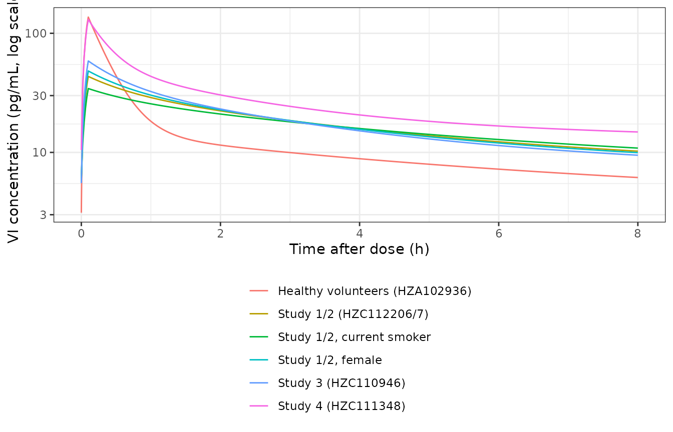

Steady-state vilanterol plasma concentration over one 24 h dosing interval after 25 ug once daily, by study stratum and covariate contrast. Compare with Fig. 4 of Siederer 2016 (VPC stratified by study).

Non-compartmental analysis

vi_conc <- vi_sim |>
  filter(!is.na(Cc)) |>
  transmute(
    id = factor(id), time, treatment = arm,
    Cc = Cc * NG_PER_ML_TO_PG_PER_ML
  )

vi_dose_df <- vi_events |>
  filter(evid == 1) |>
  transmute(id = factor(id), time, amt = 25, treatment = arm)

vi_conc_obj <- PKNCA::PKNCAconc(
  vi_conc, Cc ~ time | treatment + id,
  concu = "pg/mL", timeu = "h"
)
vi_dose_obj <- PKNCA::PKNCAdose(
  vi_dose_df, amt ~ time | treatment + id,
  doseu = "ug"
)

vi_nca <- PKNCA::pk.nca(
  PKNCA::PKNCAdata(
    vi_conc_obj, vi_dose_obj,
    intervals = data.frame(
      start = 0, end = 24,
      cmax = TRUE, tmax = TRUE, cmin = TRUE, auclast = TRUE, cav = TRUE
    )
  )
)

Comparison against published exposures

Siederer 2016 Table 4 reports model-predicted steady-state Cmax and AUC0-24 by study. The three COPD study strata are compared directly.

table4 <- tibble::tribble(
  ~treatment, ~cmax, ~auclast,
  "Study 1/2 (HZC112206/7)", 43.2, 273.7,
  "Study 3 (HZC110946)", 49.7, 249.2,
  "Study 4 (HZC111348)", 120.5, 408.2
)

vi_cmp <- nlmixr2lib::ncaComparisonTable(
  simulated = vi_nca,
  reference = table4,
  by = "treatment",
  params = c("cmax", "auclast"),
  units = c(cmax = "pg/mL", auclast = "pg*h/mL")
)
knitr::kable(vi_cmp, digits = 1)

NCA parameter	treatment	Reference	Simulated	% diff
Cmax (pg/mL)	Study 1/2 (HZC112206/7)	43.2	43.5	+0.6%
Cmax (pg/mL)	Study 3 (HZC110946)	49.7	58.6	+17.9%
Cmax (pg/mL)	Study 4 (HZC111348)	120	131	+8.5%
AUClast (pg*h/mL)	Study 1/2 (HZC112206/7)	274	264	-3.4%
AUClast (pg*h/mL)	Study 3 (HZC110946)	249	264	+6.0%
AUClast (pg*h/mL)	Study 4 (HZC111348)	408	421	+3.1%

attr(vi_cmp, "footnote")
#> NULL

The Study 1/2 stratum – 1002 of the 1091 COPD subjects, and the reference category that carries no study effect – reproduces to well under 5% on both parameters. That is the strict gate:

vi_pct <- vi_cmp |>
  mutate(pct = suppressWarnings(as.numeric(gsub("[^0-9.eE+-]", "", `% diff`))))

ref_rows <- vi_pct |> filter(treatment == "Study 1/2 (HZC112206/7)")
stopifnot(
  # Structural: a mis-transcribed CL/F, V1/F, D1 or dose, or a wrong
  # compartment mapping, moves these by tens of percent.
  max(abs(ref_rows$pct)) < 5
)

# The two small study strata (N = 50 and N = 39 subjects) are held to a
# looser envelope. Each simulated arm here is a single typical subject --
# a 60-year-old, 70 kg, non-smoking male -- whereas the matching Table 4
# row is a geometric mean over a cohort that is 68% female and 53% current
# smokers (Online Resource Table S2). Current smoking alone raises V1/F by
# 34% and so lowers Cmax by about a fifth, which is why the volume-driven
# Cmax rows sit high while the clearance-driven AUC rows do not.
stopifnot(max(abs(vi_pct$pct), na.rm = TRUE) < 20)

sprintf(
  "Study 1/2 reference stratum: max |%% diff| = %.1f%%; all strata: max = %.1f%%",
  max(abs(ref_rows$pct)), max(abs(vi_pct$pct), na.rm = TRUE)
)
#> [1] "Study 1/2 reference stratum: max |% diff| = 3.4%; all strata: max = 17.9%"

A sharper structural check is available for Study 3, because Siederer 2016 retains a study effect on V1/F for HZC110946 but none on CL/F. Steady-state AUC over a dosing interval depends only on clearance, so the model’s Study 3 AUC0-24 must be identical to its Studies 1/2 value. Mis-assigning the Study 3 coefficient to clearance instead of volume – an easy transcription slip, since the Study 4 coefficient acts on both – would break this immediately:

vi_summary <- as.data.frame(vi_nca$result) |>
  filter(PPTESTCD %in% c("cmax", "auclast")) |>
  select(treatment, PPTESTCD, PPORRES) |>
  tidyr::pivot_wider(names_from = PPTESTCD, values_from = PPORRES)

auc_s12 <- vi_summary$auclast[vi_summary$treatment == "Study 1/2 (HZC112206/7)"]
auc_s3 <- vi_summary$auclast[vi_summary$treatment == "Study 3 (HZC110946)"]

sprintf(
  "AUC0-24: Studies 1/2 = %.3f, Study 3 = %.3f pg*h/mL (relative difference %.2e)",
  auc_s12, auc_s3, abs(auc_s3 - auc_s12) / auc_s12
)
#> [1] "AUC0-24: Studies 1/2 = 264.263, Study 3 = 264.259 pg*h/mL (relative difference 1.35e-05)"

# The residual is trapezoidal quadrature error: Study 3's smaller V1/F gives a
# sharper peak and so a slightly different quadrature bias. It converges O(h^2)
# -- 1.18e-5 at the 0.02 h grid used here, 5.21e-6 at 0.01 h, 1.95e-6 at
# 0.005 h. Assigning the Study 3 coefficient to clearance instead of volume
# would instead give exp(-0.358), a 43% difference, so this is a strict gate.
stopifnot(abs(auc_s3 - auc_s12) / auc_s12 < 1e-4)

# Both also sit within 3e-5 of dose / CL = 25 ug / 94.6 L/h, so vilanterol
# satisfies the same steady-state mass-balance identity checked for
# fluticasone furoate above.
stopifnot(abs(auc_s12 - 1000 * 25 / 94.6) / (1000 * 25 / 94.6) < 1e-4)

Table 4 nevertheless reports 273.7 and 249.2 pg*h/mL for those two strata, a 9% spread the final model attributes to nothing – a reminder that Table 4 rows are summaries of post hoc individual estimates in cohorts of very different size (N = 496 and N = 50), not model predictions at a common covariate vector.

The Study 4 contrast that Sect. 4 highlights is also reproduced:

vi_summary <- as.data.frame(vi_nca$result) |>
  filter(PPTESTCD %in% c("cmax", "auclast")) |>
  select(treatment, PPTESTCD, PPORRES) |>
  tidyr::pivot_wider(names_from = PPTESTCD, values_from = PPORRES)

s12 <- vi_summary |> filter(treatment == "Study 1/2 (HZC112206/7)")
s4 <- vi_summary |> filter(treatment == "Study 4 (HZC111348)")

tibble::tibble(
  Contrast = c("Cmax, Study 4 / Study 1-2", "AUC0-24, Study 4 / Study 1-2"),
  `Sect. 4` = c("~2.7-fold", "~1.5-fold"),
  Model = c(s4$cmax / s12$cmax, s4$auclast / s12$auclast)
) |>
  knitr::kable(digits = 2)

Contrast	Sect. 4	Model
Cmax, Study 4 / Study 1-2	~2.7-fold	3.01
AUC0-24, Study 4 / Study 1-2	~1.5-fold	1.59


stopifnot(
  s4$cmax / s12$cmax > 2.5, s4$cmax / s12$cmax < 3.2,
  s4$auclast / s12$auclast > 1.4, s4$auclast / s12$auclast < 1.8
)

Smoking and sex contrasts

Table 4 also summarises exposure by sex and smoking status. These rows pool all studies and all covariate values, so they are not clean isolations of the model coefficient – they are marginal summaries over a cohort in which age, weight and study membership also differ between the strata.

contrast_tbl <- vi_summary |>
  filter(treatment %in% c(
    "Study 1/2 (HZC112206/7)", "Study 1/2, female", "Study 1/2, current smoker"
  ))

base <- contrast_tbl |> filter(treatment == "Study 1/2 (HZC112206/7)")
fem <- contrast_tbl |> filter(treatment == "Study 1/2, female")
smk <- contrast_tbl |> filter(treatment == "Study 1/2, current smoker")

tibble::tibble(
  Contrast = c("Cmax, female / male", "Cmax, current / former smoker"),
  `Table 4 (marginal)` = c(42.1 / 45.7, 38.3 / 49.4),
  `Model (all else equal)` = c(fem$cmax / base$cmax, smk$cmax / base$cmax)
) |>
  knitr::kable(digits = 3)

Contrast	Table 4 (marginal)	Model (all else equal)
Cmax, female / male	0.921	1.111
Cmax, current / former smoker	0.775	0.791

The smoking contrast survives marginalisation almost intact – Table 4 gives 0.775 and Sect. 4 quotes “22 %” lower Cmax in current smokers, against 0.746 all-else-equal from the model. The sex contrast does not: holding everything else fixed the model predicts females have a higher Cmax (12% lower V1/F), yet Table 4’s marginal female/male ratio is 0.92. The paper reaches the same conclusion from its own numbers – Sect. 4: “there appeared to be no notable difference in VI systemic exposure for males compared with females (Table 4)”. A marginal summary over a cohort whose strata differ in several correlated covariates can mask and even invert a single covariate’s effect, so only the isolated coefficient (checked above against Table 2) is gated.

Covariate-driven cohort

With no estimable IIV, all between-subject variability in this model comes from the covariates. A virtual COPD cohort sampled over the Table S2 demographic ranges shows the spread the covariate model alone produces, which is the quantity Online Resource Fig. S2 plots.

set.seed(20260916)
n_cohort <- 200

cohort <- tibble::tibble(
  id = seq_len(n_cohort),
  AGE = round(runif(n_cohort, 41, 84)),
  WT = round(rlnorm(n_cohort, meanlog = log(73), sdlog = 0.22)),
  SEXF = rbinom(n_cohort, 1, 0.68),
  SMOKE = rbinom(n_cohort, 1, 0.53),
  DIS_COPD = 1,
  STUDY_HZC110946 = 0,
  STUDY_HZC111348 = 0
) |>
  mutate(WT = pmin(pmax(WT, 35), 160))

cohort_events <- cohort |>
  group_split(id) |>
  lapply(function(g) {
    dplyr::bind_rows(
      data.frame(
        id = g$id, time = 0, amt = 25, evid = 1, cmt = "central",
        rate = -2, ii = 24, ss = 1
      ),
      data.frame(
        id = g$id, time = seq(0, 24, by = 0.1), amt = NA_real_, evid = 0,
        cmt = "central", rate = 0, ii = 0, ss = 0
      )
    )
  }) |>
  dplyr::bind_rows() |>
  left_join(cohort, by = "id") |>
  arrange(id, time, dplyr::desc(evid))

cohort_sim <- rxode2::rxSolve(
  vi, cohort_events, keep = c("AGE", "WT", "SEXF", "SMOKE"),
  returnType = "data.frame"
)
#> ℹ omega/sigma items treated as zero: 'etalcl', 'etalvp2'
#> Warning: multi-subject simulation without without 'omega'

cohort_exposure <- cohort_sim |>
  filter(!is.na(Cc)) |>
  group_by(id, AGE, WT) |>
  summarise(
    cmax = max(Cc) * NG_PER_ML_TO_PG_PER_ML,
    auc = sum(diff(time) * (head(Cc, -1) + tail(Cc, -1)) / 2) *
      NG_PER_ML_TO_PG_PER_ML,
    .groups = "drop"
  )

cohort_exposure |>
  tidyr::pivot_longer(c(cmax, auc), names_to = "param", values_to = "value") |>
  tidyr::pivot_longer(c(AGE, WT), names_to = "cov", values_to = "cov_value") |>
  mutate(
    param = dplyr::recode(param, cmax = "Cmax (pg/mL)", auc = "AUC0-24 (pg*h/mL)"),
    cov = dplyr::recode(cov, AGE = "Age (years)", WT = "Weight (kg)")
  ) |>
  ggplot(aes(cov_value, value)) +
  geom_point(alpha = 0.4) +
  geom_smooth(method = "loess", formula = y ~ x, se = FALSE) +
  facet_grid(param ~ cov, scales = "free") +
  labs(x = NULL, y = NULL) +
  theme_bw()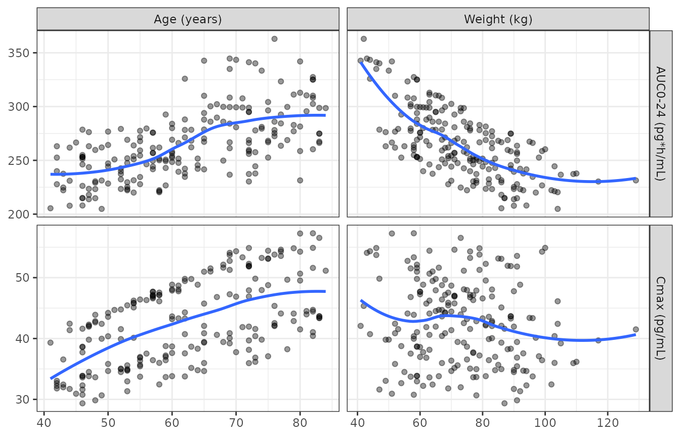

Steady-state vilanterol AUC0-24 and Cmax against age and bodyweight in a 200-subject virtual COPD cohort. Replicates Online Resource Fig. S2 of Siederer 2016.

tibble::tibble(
  Statistic = c("Geometric mean", "5th percentile", "95th percentile"),
  `Cmax (pg/mL)` = c(
    exp(mean(log(cohort_exposure$cmax))),
    quantile(cohort_exposure$cmax, 0.05),
    quantile(cohort_exposure$cmax, 0.95)
  ),
  `AUC0-24 (pg*h/mL)` = c(
    exp(mean(log(cohort_exposure$auc))),
    quantile(cohort_exposure$auc, 0.05),
    quantile(cohort_exposure$auc, 0.95)
  )
) |>
  knitr::kable(digits = 1)

Statistic	Cmax (pg/mL)	AUC0-24 (pg*h/mL)
Geometric mean	42.0	263.2
5th percentile	32.2	220.4
95th percentile	54.3	326.0


# Centre of the covariate-driven cohort against Table 4 'All studies'
# (Cmax 43.2 pg/mL, AUC0-24 265.7 pg*h/mL). Robust to the sampled cohort,
# because the assertion is on the geometric mean, not on an extreme.
gm_auc <- exp(mean(log(cohort_exposure$auc)))
stopifnot(abs(gm_auc - 265.7) / 265.7 < 0.15)
sprintf("Cohort geometric-mean AUC0-24 %.1f vs Table 4 'All studies' 265.7 pg*h/mL", gm_auc)
#> [1] "Cohort geometric-mean AUC0-24 263.2 vs Table 4 'All studies' 265.7 pg*h/mL"

Sect. 4 notes “there was no notable trend in predicted systemic exposure with increasing age or decreasing bodyweight”, and the loess curves above show why: age lowers CL/F (raising AUC) and V1/F (raising Cmax) simultaneously, while weight raises CL/F, so the net covariate-driven spread in exposure is modest relative to the between-study difference.

Assumptions and deviations

Errata and corrections applied

1. The continuous-covariate equation is printed without its inner logarithm. Siederer 2016 Sect. 3.2.2 prints

Ln CL = theta_1 + theta_COV x (covariate / median)

but the model files implement the power form

Ln P = theta_1 + theta_COV x Ln(covariate / reference)

Three independent statements in the paper falsify the printed form and confirm the power form:

Sect. 3.2.2 quotes “a reduction (47 %) in inhaled clearance … with decreasing bodyweight (range of 160-35 kg)”. The power form gives exp(0.421 * log(35/160)) = 0.527, a 47.3% reduction. The printed linear-ratio form gives exp(0.421 * (35 - 160)/70) = 0.471, a 52.9% reduction.
exp(4.55) = 94.6 L/h is quoted as the typical CL/F at exactly 60 years and 70 kg, and exp(6.46) = 639 L as the typical V1/F at exactly 60 years. Both require the covariate term to vanish at the reference, which only the power form does; the printed form would leave theta_COV x 1 behind and give 93.5 L/h and 388 L instead.
Sect. 3.2.2 quotes a 30% decrease in V1/F over 41-84 years; the power form gives exp(-0.499 * log(84/41)) = 0.699.

The gate in “Typical parameter values” above re-runs all of these on every render, so the correction cannot silently regress.

2. Reference values for the power model are 60 years and 70 kg, taken from the Sect. 3.2.2 typical-value statements (“a subject with COPD (aged 60 years and weighing 70 kg)”; “non-smoking male, aged 60 years”). The word used in the printed equation is “median”, and Online Resource Table S2 gives a median age of 61.0 years and a mean weight of 75.3 kg for the VI dataset, so the model’s reference values are the rounded standards the results text uses rather than the tabulated dataset statistics. Using 61 y / 75.3 kg would shift exp(theta_1) away from the paper’s own quoted typical values.

3. Table 2’s V3/F row header misprints the unit as L/h. The table footnote (“V2/F, V3/F volumes of peripheral compartment”) and dimensional analysis both confirm it is a volume (L). Encoded as a volume.

4. Table 2’s D1 footnote reads “input duration as FF/VI or FF alone” in a vilanterol parameter table. D1 is the vilanterol zero-order input duration; the footnote text appears to have been copied from the fluticasone furoate table.

5. Fluticasone furoate Table 1 and Table 3 are mutually inconsistent by a factor of roughly 2.4-2.7 on AUC. This is the largest deviation in the extraction and it is not resolvable from the sources on disk, so nothing was tuned.

Table 1 is internally consistent four ways: its “Ln estimate” and “Estimate” columns are exact exponentials of each other, its confidence intervals agree, and it reproduces all four typical CL/F values quoted in Sect. 3.1.2 (230, 186, 244, 176 L/h) exactly – see the gate in “Typical clearance by race category”.
The model built from Table 1 satisfies the steady-state mass-balance identity AUC(0-tau) = dose / CL to machine precision, so the ODE system, compartment mapping and unit declaration are correct.
Nonetheless the model predicts steady-state AUC0-24 that is 2.6x, 2.4x and 2.7x higher than Table 3’s model-predicted exposures at 50, 100 and 200 ug respectively. At the 100 ug stratum – which holds 724 of Table 3’s subject-dose records and is by far the best determined – the offset is a clean scale factor: 2.388x on Cmax and 2.391x on AUC, leaving Table 3’s own AUC/Cmax ratio of 15.50 h essentially identical to the model’s 15.52 h. The profile shape therefore agrees and only the dose-to-clearance scale differs. Reproducing Table 3’s absolute numbers at 100 ug would require CL/F = 549 L/h, or an effective FF dose of 41.9 ug in place of 100 ug; neither appears anywhere in the paper. The emitted-dose footnote in Online Resource Table S1 (“Emitted doses 46/22, 92/22, 184/22 and 368/22 ug”) accounts for only a factor of 1.09.
The offset is not perfectly constant across doses, because Table 3 is itself not dose-proportional: its AUC rises 2.19-fold from 50 to 100 ug and 1.76-fold from 100 to 200 ug, whereas a linear model is exactly dose-proportional. Some departure is expected – Sect. 2.5 defines AUC0-24 as nominal dose divided by each subject’s post hoc CL/F, and the dose groups contain different subjects with different race mixes – but it means no single constant reconciles Table 3 with any linear model. The 50 ug stratum deviates most (AUC/Cmax 11.0 h against the model’s 15.5 h), which is consistent with Sect. 3.1.1’s report that 72% of its samples were below the limit of quantification.
The equivalent check for vilanterol passes cleanly: Table 2’s exp(4.55) = 94.6 L/h and a 25 ug dose give 264.3 pg*h/mL against Table 4’s “All studies” geometric mean of 265.7 pg*h/mL, a 0.5% agreement. So the inconsistency is specific to the fluticasone furoate analysis, not a systematic units error across the paper.
The paper’s own visual predictive check sides with Table 1. Fig. 2 panel
1. is the 100 ug stratum, plotted on a linear pg/mL axis. Its observed concentration cloud spans roughly 0-90 pg/mL with the observed median running from about 45 pg/mL early in the interval down to about 25 pg/mL at 24 h, and the model prediction intervals bracket it. A geometric-mean Cmax of 11.73 pg/mL and Cavg of 7.6 pg/mL – what Table 3 reports for that same 100 ug stratum – cannot be reconciled with that figure, whereas the Table 1 model simulated here (Cmax 28.0 pg/mL, Cavg 18.1 pg/mL) sits inside it. Table 3, not Table 1, is the outlier.
The model file therefore encodes Table 1, which is the paper’s stated final parameter table and the only self-consistent description of the model. Users reproducing Table 3’s absolute exposures should be aware that Table 3 cannot be regenerated from Table 1. Sect. 3.1.2 notes that the 50/25 ug treatment was excluded during model building and that “this model and the base model were re-run including all treatments” afterwards; if Table 1 and Table 3 come from the two different runs, that would explain a systematic offset, but the paper does not say so.

Parameters not reported by the source

Inter-individual variability magnitudes are not reported anywhere. Both Sect. 3.1.2 and Sect. 3.2.2 state that “Inter-individual variances (exponential model) were estimated with reasonable precision” and give only %RSE bounds (<= 36% for FF, <= 25% for VI except V3/F at 64%). Neither Table 1, Table 2 nor the Online Resource lists an OMEGA row. Per project policy, no variance was invented. Instead, etas are declared at fixed(0) on only the parameters for which the paper gives positive evidence of an estimated IIV:

FF: etalcl, because Sect. 2.5 derives “individual post hoc estimates of CL/F”.
VI: etalcl for the same reason, and etalvp2, named explicitly in Sect. 3.2.2 (“ETA on volume of the peripheral compartment (V3/F) where %RSE was 64 %”).

Consequently both models are deterministic: simulated between-subject variability comes only from covariates. Every gate in this vignette is an exact comparison rather than a distributional one, which is why tight tolerances are used throughout. Anyone needing a stochastic simulation must supply their own omega.

Residual-error magnitudes are not reported either, so addSd (FF) and expSd (VI) are also fixed(0).

The residual-error scale differs between the two models, and the paper does not say so in prose – both simply say “An additive error model described the residual variability.” The figures settle it: Fig. 1 (FF goodness-of-fit) has axes “Observed FF Concentration (pg/mL)” against “Population Prediction (pg/mL)”, untransformed, so FF’s additive error is additive in pg/mL and maps to add(). Fig. 3 (VI goodness-of-fit) has axes “Observed log-Value (pg/mL)” against “Population log-Prediction (pg/mL)”, and the Fig. 4 VPC axis is “LN concentration (pg/mL)”, so VI was fitted on the natural-log concentration scale and its additive error is log-normal in linear space, mapping to lnorm().

VI residual error was separated by population (Sect. 3.2.2: “CL/F, V1/F, volume of the peripheral compartment (V2/F), and residual error were separated by population”). Neither stratum’s magnitude is reported, so a single expSd is declared.

Which VI parameters carried fixed IIV in the base model is stated but not quantified. Sect. 3.2.2 notes “inter-subject variability on D1, Q2/F, and V2/F was fixed”, without giving the fixed values, and describes the structural base model rather than the final model.

Other assumptions

Race grouping. Siederer 2016’s RACE1 is a paper-defined collapse of a nine-level race column driven by small per-category N (Sect. 2.3.1). Its groupings do not correspond to any race indicator already in the nlmixr2lib covariate register, so two new composite covariates were registered: RACE_ASIAN_EAST_SE (RACE1 = 2) and RACE_ASIAN_CENTRAL_ARABIC_AMIND_OTH (RACE1 = 4). RACE1 = 3 maps onto the existing RACE_BLACK. All three are mutually exclusive and all three = 0 selects the White/Caucasian reference. Note in particular that RACE1 = 2 excludes Central/South Asian heritage (which falls in RACE1 = 4), so it is not RACE_ASIAN, and it includes South East Asian heritage, so it is not RACE_ASIAN_NORTHEAST.
Smoking reference category. All Phase II/III subjects had at least 10 pack-years at screening (Sect. 2.1), so the covariate is current-vs-former smoker and the canonical SMOKE indicator is used (reference = former smoker), not the three-level SMOKE_CURRENT / SMOKE_NEVER pair.
Sex coding. The paper codes males = 1, females = 2 and applies theta_COV x (covariate - 1), so SEXF = source code - 1 and the coefficient applies exactly when SEXF = 1.
Covariates apply to COPD subjects only. Every covariate row in Table 2 is labelled “COPD”, and Sect. 3.2.2 introduces them “for subjects with COPD”, so the model gates all of them on DIS_COPD.
Doses are nominal, not emitted. Sect. 2.5 derives AUC0-24 as “ratio of nominal dose/individual post hoc estimate of CL/F”, and the vilanterol reproduction above confirms nominal dosing (25 ug / 94.6 L/h = 264.3 vs Table 4’s 265.7 pg*h/mL; the emitted dose of 22 ug would give 232.6).
Study effects are encoded as protocol-numbered indicators (STUDY_HZC110946, STUDY_HZC111348) rather than the paper’s “Study 3” / “Study 4” labels, using the mapping in Online Resource Table S1, so the covariate names are unambiguous outside the context of this paper.
The healthy-volunteer stratum has no covariate model. Table 2 reports separate CL/F, V1/F and V2/F for healthy volunteers and no covariate effects for them, so the age/weight/sex/smoking/study terms are switched off when DIS_COPD = 0.
Q2/F, Q3/F, V3/F and D1 are shared across the COPD and healthy strata, because Table 2 reports a single estimate for each.