Cyclophosphamide brain ECF (Campagne 2019, mouse)
Source:vignettes/articles/Campagne_2019_cyclophosphamide_mouse.Rmd
Campagne_2019_cyclophosphamide_mouse.RmdModel and source
- Citation: Campagne O, Davis A, Zhong B, Nair S, Haberman V, Patel YT, Janke L, Roussel MF, Stewart CF. CNS Penetration of Cyclophosphamide and Metabolites in Mice Bearing Group 3 Medulloblastoma and Non-Tumor Bearing Mice. J Pharm Pharm Sci. 2019;22(1):553-568.
- Article (open access): https://doi.org/10.18433/jpps30608
Cyclophosphamide (CTX) is an alkylating prodrug widely used for pediatric brain tumors. It is hydroxylated in the liver to the activated metabolite 4-hydroxy-cyclophosphamide (4OH-CTX), which tautomerises to aldophosphamide and is then oxidised to the downstream inactive metabolite carboxyethylphosphoramide mustard (CEPM). Campagne 2019 used cerebral microdialysis in CD-1 nude mice (non-tumor-bearing and orthotopic Group 3 medulloblastoma) to characterise the brain/tumor extracellular fluid (ECF) penetration of CTX and its two metabolites after a single 130 mg/kg IP dose. The packaged model jointly describes six analyte profiles:
-
CTX plasma (output
Cc): two-compartment plasma model with linear elimination representing CTX -> 4OH-CTX hydroxylation. -
4OH-CTX plasma (output
Cc_4ohctx): apparent two-compartment plasma model (apparent CL/Fm, V/Fm with Fm = 1). -
CEPM plasma (output
Cc_cepm): apparent two-compartment plasma model. -
CTX brain/tumor ECF (output
Cecf): one-compartment ECF linked to plasma central via influx clearance (CLin, drives FU x Cp into ECF) and efflux clearance (CLef, drives Cecf back to plasma). -
4OH-CTX brain/tumor ECF (output
Cecf_4ohctx): same structure. -
CEPM brain/tumor ECF (output
Cecf_cepm): same structure.
The ECF compartment volume is fixed to 0.001 L/kg (ref 26 of Campagne 2019) and plasma fraction unbound (FU) is fixed to the in-vitro equilibrium-dialysis median for each compound. The cascade is parameterised in molar units (umol/kg dose, uM concentration) so the 1:1 stoichiometric conversion CTX -> 4OH-CTX -> CEPM is preserved without molecular-weight scaling.
mod_obj <- rxode2::rxode(readModelDb("Campagne_2019_cyclophosphamide_mouse"))
#> ℹ parameter labels from comments will be replaced by 'label()'
str(mod_obj$population, max.level = 1)
#> List of 10
#>  $ species       : chr "mouse (CD-1 nude, female)"
#>  $ n_subjects    : int 41
#>  $ n_studies     : int 5
#>  $ sex_female_pct: num 100
#>  $ disease_state : chr "Non-tumor-bearing (NTB) and orthotopic Group 3 medulloblastoma (G3MB, 1e5 luciferase-transduced cells stereotac"| __truncated__
#>  $ dose_range    : chr "130 mg/kg cyclophosphamide IP single dose (498 umol/kg using MW = 261.09 g/mol)."
#>  $ regions       : chr "USA (St. Jude Children's Research Hospital)."
#>  $ n_observations: chr "Plasma: 30 samples in the plasma-only study + 14 + 23 + 27 + 21 = 115 samples across the four microdialysis stu"| __truncated__
#>  $ cohorts       : chr "Plasma-only PK study: 12 NTB mice with sparse sampling at 5 min, 0.25, 0.5, 1, 1.5, 2, 4, 6 h. Microdialysis st"| __truncated__
#>  $ notes         : chr "Plasma model parameters (Campagne 2019 Table 2 upper block) were estimated from pooled plasma data from all fiv"| __truncated__
Population
Campagne 2019 pooled data from five studies in female CD-1 nude mice given 130 mg/kg cyclophosphamide IP as a single dose (Table 1):
- a plasma-only PK study (n = 12 non-tumor-bearing) with sparse plasma sampling at 5 min, 0.25, 0.5, 1, 1.5, 2, 4, and 6 h post-dose;
- four cerebral microdialysis studies that combined sparse plasma sampling (0.25, 1, 2 h limited-sampling design) with hourly ECF collection over 5 h: M1 (n = 5 NTB) and M2 (n = 8 G3MB) used a phenylhydrazine derivatizing solution directly in the perfusate; M3 (n = 9 NTB) and M4 (n = 7 G3MB) used the derivatizing solution in the dialysate collection tubes instead.
Histology after M1/M2 showed substantial brain hemorrhage and necrosis around the probe site (mean 18% and 17% of brain sections affected, respectively), which led the authors to drop the M1/M2 ECF data from the final fit. The plasma data from all five studies (41 mice total) contributed to the plasma sub-model; only M3 + M4 ECF data (16 mice) contributed to the ECF sub-model. No covariates were retained in the structural model – tumor status was analysed post hoc on individual Kp,uu rather than as a model effect, and the final plasma and ECF parameters in Campagne 2019 Table 2 are a single pooled set across NTB and G3MB mice.
Source trace
The per-parameter origin is recorded as an in-file comment next to
each ini() entry in
inst/modeldb/specificDrugs/Campagne_2019_cyclophosphamide_mouse.R.
The table below collects them in one place for review.
| Equation / parameter | Value | Source location |
|---|---|---|
lcl (CTX CL) |
log(4.4) L/h/kg | Campagne 2019 Table 2 (3.7% RSE) |
lvc (CTX V) |
log(0.65) L/kg | Campagne 2019 Table 2 (5.0% RSE) |
lq (CTX Q) |
log(0.18) L/h/kg | Campagne 2019 Table 2 (4.3% RSE) |
lvp (CTX Vp) |
log(0.062) L/kg | Campagne 2019 Table 2 (2.6% RSE) |
lcl_4ohctx (4OH-CTX CL/Fm) |
log(11) L/h/kg | Campagne 2019 Table 2 (4.9% RSE) |
lvc_4ohctx (4OH-CTX V/Fm) |
log(2.4) L/kg | Campagne 2019 Table 2 (6.2% RSE) |
lq_4ohctx (4OH-CTX Q/Fm) |
log(0.075) L/h/kg | Campagne 2019 Table 2 (17% RSE) |
lvp_4ohctx (4OH-CTX Vp/Fm) |
log(0.22) L/kg | Campagne 2019 Table 2 (20% RSE) |
lcl_cepm (CEPM CL/Fm) |
log(6.4) L/h/kg | Campagne 2019 Table 2 (3.0% RSE) |
lvc_cepm (CEPM V/Fm) |
log(1.1) L/kg | Campagne 2019 Table 2 (5.3% RSE) |
lq_cepm (CEPM Q/Fm) |
log(1.6) L/h/kg | Campagne 2019 Table 2 (9.0% RSE) |
lvp_cepm (CEPM Vp/Fm) |
log(1.7) L/kg | Campagne 2019 Table 2 (7.1% RSE) |
lclin (CTX CLin) |
log(4.3e-4) L/h/kg | Campagne 2019 Table 2 (16% RSE) |
lclef (CTX CLef) |
log(2.4e-3) L/h/kg | Campagne 2019 Table 2 (7.0% RSE) |
lclin_4ohctx (4OH-CTX CLin) |
log(2.3e-4) L/h/kg | Campagne 2019 Table 2 (25% RSE) |
lclef_4ohctx (4OH-CTX CLef) |
log(3.3e-3) L/h/kg | Campagne 2019 Table 2 (4.9% RSE) |
lclin_cepm (CEPM CLin) |
log(8.8e-5) L/h/kg | Campagne 2019 Table 2 (17% RSE) |
lclef_cepm (CEPM CLef) |
log(1.5e-3) L/h/kg | Campagne 2019 Table 2 (7.2% RSE) |
lvecf (ECF volume, FIXED) |
log(0.001) L/kg | Campagne 2019 Methods, citing Stewart 2010 (ref 26) |
fu (CTX FU, FIXED) |
0.26 | Campagne 2019 Results, “Plasma protein binding studies” (median, range 0.24-0.28) |
fu_4ohctx (4OH-CTX FU, FIXED) |
0.39 | Campagne 2019 Results (median, range 0.28-0.48) |
fu_cepm (CEPM FU, FIXED) |
0.31 | Campagne 2019 Results (median, range 0.29-0.34) |
etalcl (eta-CL_CTX) |
SD = 0.11 -> var = 0.0121 | Campagne 2019 Table 2 (17% RSE) |
etalcl_4ohctx (eta-CL_4OH-CTX) |
SD = 0.13 -> var = 0.0169 | Campagne 2019 Table 2 (19% RSE) |
etalcl_cepm (eta-CL_CEPM) |
SD = 0.094 -> var = 0.008836 | Campagne 2019 Table 2 (25% RSE) |
etalvc_cepm (eta-V_CEPM) |
SD = 0.22 -> var = 0.0484 | Campagne 2019 Table 2 (21% RSE) |
etalclin (eta-CLin_CTX) |
SD = 0.31 -> var = 0.0961 | Campagne 2019 Table 2 (51% RSE) |
etalclef (eta-CLef_CTX) |
SD = 0.23 -> var = 0.0529 | Campagne 2019 Table 2 (22% RSE) |
etalclin_4ohctx (eta-CLin_4OH-CTX) |
SD = 0.86 -> var = 0.7396 | Campagne 2019 Table 2 (19% RSE) |
etalclin_cepm (eta-CLin_CEPM) |
SD = 0.62 -> var = 0.3844 | Campagne 2019 Table 2 (19% RSE) |
etalclef_cepm (eta-CLef_CEPM) |
SD = 0.20 -> var = 0.04 | Campagne 2019 Table 2 (38% RSE) |
propSd (CTX plasma RUV) |
0.24 | Campagne 2019 Table 2 (11% RSE) |
propSd_4ohctx (4OH-CTX plasma RUV) |
0.29 | Campagne 2019 Table 2 (11% RSE) |
propSd_cepm (CEPM plasma RUV) |
0.18 | Campagne 2019 Table 2 (12% RSE) |
propSd_Cecf (CTX ECF RUV) |
0.45 | Campagne 2019 Table 2 (12% RSE) |
propSd_Cecf_4ohctx (4OH-CTX ECF RUV) |
0.33 | Campagne 2019 Table 2 (16% RSE) |
propSd_Cecf_cepm (CEPM ECF RUV) |
0.22 | Campagne 2019 Table 2 (15% RSE) |
| ODE: 3 sequential 2-cmt plasma + 3 ECF (1-cmt each) | n/a | Campagne 2019 Methods “Tumor and brain ECF pharmacokinetic modeling” and Figure 1 |
IP dose modelled as bolus into central (no absorption
compartment) |
n/a | Campagne 2019 Figure 1 (no Ka in structure) |
| Sequential metabolism CTX -> 4OH-CTX -> CEPM with Fm = 1 | n/a | Campagne 2019 Results “Plasma pharmacokinetics” |
| BBB transfer driven by FU x Cp into ECF | n/a | Campagne 2019 Methods “the amount of drug in the plasma was multiplied by the corresponding FU” |
Virtual cohort
We simulate the 16 microdialysis mice (M3 NTB and M4 G3MB cohorts) that contributed to the ECF fit. The structural model has no cohort effect, so NTB and G3MB mice are biologically identical in this implementation; the cohort label is carried only for cohort-stratified summaries against the paper’s Table 3 entries.
set.seed(20191204) # Campagne 2019 publication date

# Dose conversion: 130 mg/kg cyclophosphamide / 261.09 g/mol = 498 umol/kg.
mw_ctx <- 261.09
dose_mg_per_kg <- 130
dose_umol_per_kg <- dose_mg_per_kg / mw_ctx * 1000  # ~497.9 umol/kg

# Build one cohort with disjoint IDs so multiple cohorts can be bind_rows()-ed.
make_cohort <- function(n, cohort, id_offset = 0L) {
  ids <- id_offset + seq_len(n)
  tibble(id = ids, cohort = cohort)
}

cohort_df <- bind_rows(
  make_cohort(9L, "M3 (NTB)",  id_offset =   0L),
  make_cohort(7L, "M4 (G3MB)", id_offset = 100L)
)

# Dosing + observation event table. Use the paper's M3/M4 limited-sampling
# plasma schedule for plasma and the hourly ECF collection schedule for ECF.
sample_times <- c(0.083, 0.25, 0.5, 1, 1.5, 2, 3, 4, 5)
events <- bind_rows(
  # one dosing event per subject at t = 0 into central
  cohort_df |>
    mutate(time = 0, amt = dose_umol_per_kg, evid = 1L, cmt = "central"),
  # observation rows: replicate sample times per subject, use 'Cc' as cmt so
  # rxode2 can assign a valid output mapping; all six outputs are written
  # at every row of the simulation regardless of which cmt is named.
  expand_grid(cohort_df, time = sample_times) |>
    mutate(amt = NA_real_, evid = 0L, cmt = "Cc")
)
stopifnot(!anyDuplicated(unique(events[, c("id", "time", "evid")])))
Simulation
mod <- readModelDb("Campagne_2019_cyclophosphamide_mouse")

# Stochastic simulation with the published IIV for a realistic VPC.
sim <- rxode2::rxSolve(mod, events = events, keep = c("cohort")) |>
  as.data.frame()
#> ℹ parameter labels from comments will be replaced by 'label()'

# Typical-value reference trajectory (no IIV) for the published-figure overlay.
mod_typical <- rxode2::zeroRe(mod)
#> ℹ parameter labels from comments will be replaced by 'label()'
typical_times <- c(0, seq(0.05, 5, length.out = 200))
typical_events <- bind_rows(
  tibble(id = 1L, time = 0, amt = dose_umol_per_kg, evid = 1L, cmt = "central"),
  tibble(id = 1L, time = typical_times, amt = NA_real_, evid = 0L, cmt = "Cc")
)
typical <- rxode2::rxSolve(mod_typical, events = typical_events) |>
  as.data.frame()
#> ℹ omega/sigma items treated as zero: 'etalcl', 'etalcl_4ohctx', 'etalcl_cepm', 'etalvc_cepm', 'etalclin', 'etalclef', 'etalclin_4ohctx', 'etalclin_cepm', 'etalclef_cepm'
Replicate published figures
Figure 2 (column 1) – plasma VPC
plasma_long <- typical |>
  select(time, Cc, Cc_4ohctx, Cc_cepm) |>
  pivot_longer(-time, names_to = "analyte", values_to = "concentration") |>
  mutate(analyte = recode(analyte,
                          Cc = "CTX", Cc_4ohctx = "4OH-CTX", Cc_cepm = "CEPM"))

ggplot(plasma_long, aes(time, concentration, colour = analyte)) +
  geom_line(linewidth = 1) +
  scale_y_log10() +
  scale_colour_manual(values = c(CTX = "#1f77b4", `4OH-CTX` = "#2ca02c",
                                  CEPM = "#d62728")) +
  labs(x = "Time (h)", y = "Plasma concentration (uM, log scale)",
       colour = NULL,
       title = "Plasma concentration-time profiles (typical values)",
       caption = paste0("Replicates the central-tendency curves shown in ",
                        "Campagne 2019 Figure 2 column 1."))
#> Warning in scale_y_log10(): log-10 transformation introduced infinite values.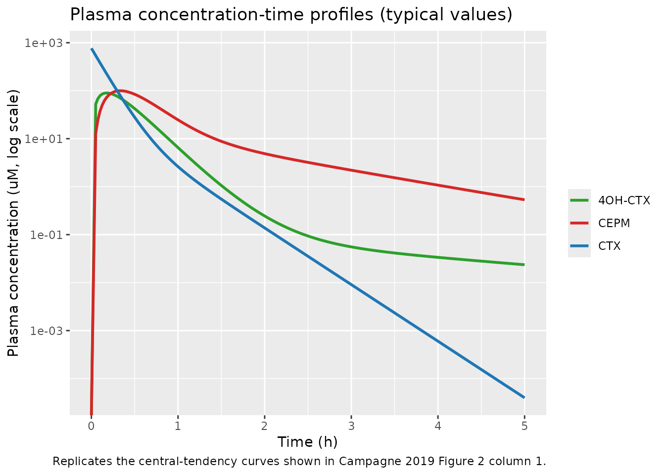
Figure 2 (column 2) – brain/tumor ECF VPC
ecf_long <- typical |>
  select(time, Cecf, Cecf_4ohctx, Cecf_cepm) |>
  pivot_longer(-time, names_to = "analyte", values_to = "concentration") |>
  mutate(analyte = recode(analyte,
                          Cecf = "CTX", Cecf_4ohctx = "4OH-CTX",
                          Cecf_cepm = "CEPM"))

ggplot(ecf_long, aes(time, concentration, colour = analyte)) +
  geom_line(linewidth = 1) +
  scale_colour_manual(values = c(CTX = "#1f77b4", `4OH-CTX` = "#2ca02c",
                                  CEPM = "#d62728")) +
  labs(x = "Time (h)", y = "Brain/tumor ECF concentration (uM)",
       colour = NULL,
       title = "Brain/tumor ECF concentration-time profiles (typical values)",
       caption = paste0("Replicates the central-tendency curves shown in ",
                        "Campagne 2019 Figure 2 column 2."))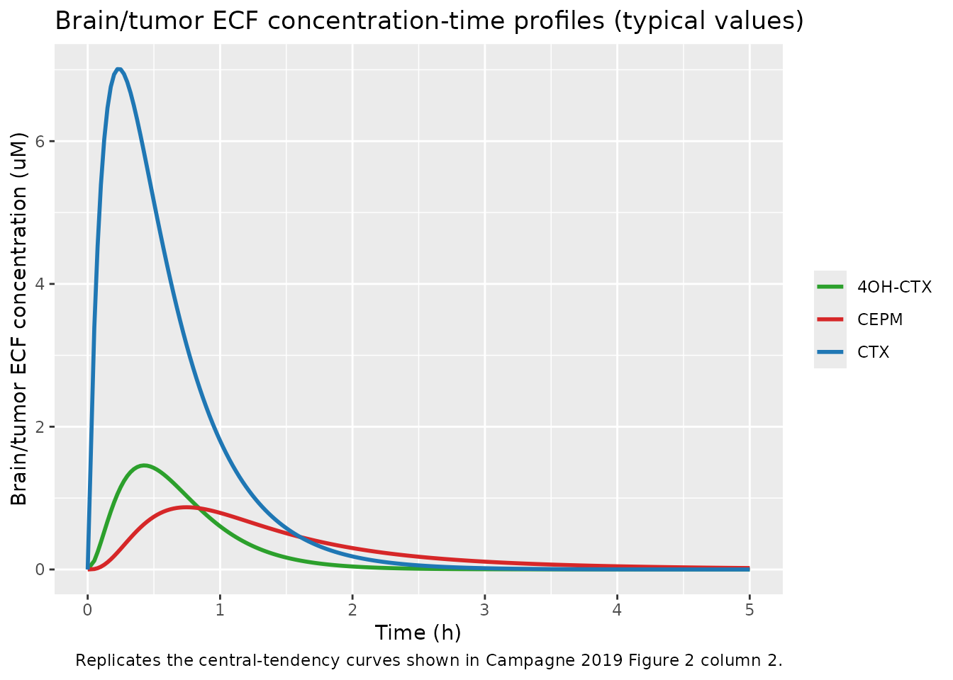
PKNCA validation
The source paper integrates AUC over 0-5 h on the model-derived
concentration-time curves for each mouse (Methods “Pharmacokinetic
modeling General methods”). PKNCA reproduces that integration with the
standard NCA plumbing. Three plasma outputs (Cc,
Cc_4ohctx, Cc_cepm) and three ECF outputs
(Cecf, Cecf_4ohctx, Cecf_cepm)
are validated; one PKNCA block per output, each with a
cohort + id grouping.
# Helper: build a PKNCAdata for one output column, scoped to 0-5 h with
# AUClast as the primary endpoint (matches the AUC0-5h definition in
# Campagne 2019 Methods). Concentrations are in uM, dose in umol/kg.
nca_for_output <- function(sim_df, dose_df, conc_col) {
  conc <- sim_df |>
    filter(!is.na(.data[[conc_col]])) |>
    select(id, time, cohort, !!conc_col)
  names(conc)[ncol(conc)] <- "Cc"
  conc_obj <- PKNCA::PKNCAconc(conc, Cc ~ time | cohort + id,
                                concu = "uM", timeu = "h")
  dose_obj <- PKNCA::PKNCAdose(dose_df, amt ~ time | cohort + id,
                                doseu = "umol/kg")
  intervals <- data.frame(
    start    = 0,
    end      = 5,
    cmax     = TRUE,
    tmax     = TRUE,
    auclast  = TRUE
  )
  res <- PKNCA::pk.nca(PKNCA::PKNCAdata(conc_obj, dose_obj,
                                        intervals = intervals))
  as.data.frame(res$result)
}

dose_df <- events |>
  filter(evid == 1L) |>
  select(id, time, amt, cohort)
nca_plasma <- bind_rows(
  nca_for_output(sim, dose_df, "Cc")        |> mutate(analyte = "CTX"),
  nca_for_output(sim, dose_df, "Cc_4ohctx") |> mutate(analyte = "4OH-CTX"),
  nca_for_output(sim, dose_df, "Cc_cepm")   |> mutate(analyte = "CEPM")
)
plasma_summary <- nca_plasma |>
  filter(PPTESTCD %in% c("cmax", "tmax", "auclast")) |>
  group_by(analyte, PPTESTCD) |>
  summarise(median = round(median(PPORRES, na.rm = TRUE), 3),
            q05 = round(quantile(PPORRES, 0.05, na.rm = TRUE), 3),
            q95 = round(quantile(PPORRES, 0.95, na.rm = TRUE), 3),
            .groups = "drop")
knitr::kable(plasma_summary,
caption = "Simulated plasma NCA (16 virtual mice, M3 + M4) at the typical-value parameter set with IIV; median (5th, 95th percentiles).")| analyte | PPTESTCD | median | q05 | q95 |
|---|---|---|---|---|
| 4OH-CTX | auclast | NA | NA | NA |
| 4OH-CTX | cmax | 83.385 | 78.318 | 94.948 |
| 4OH-CTX | tmax | 0.250 | 0.208 | 0.250 |
| CEPM | auclast | NA | NA | NA |
| CEPM | cmax | 94.107 | 74.992 | 111.033 |
| CEPM | tmax | 0.250 | 0.250 | 0.500 |
| CTX | auclast | NA | NA | NA |
| CTX | cmax | 427.652 | 373.287 | 448.518 |
| CTX | tmax | 0.083 | 0.083 | 0.083 |
nca_ecf <- bind_rows(
  nca_for_output(sim, dose_df, "Cecf")        |> mutate(analyte = "CTX"),
  nca_for_output(sim, dose_df, "Cecf_4ohctx") |> mutate(analyte = "4OH-CTX"),
  nca_for_output(sim, dose_df, "Cecf_cepm")   |> mutate(analyte = "CEPM")
)
ecf_summary <- nca_ecf |>
  filter(PPTESTCD %in% c("cmax", "tmax", "auclast")) |>
  group_by(analyte, PPTESTCD) |>
  summarise(median = round(median(PPORRES, na.rm = TRUE), 3),
            q05 = round(quantile(PPORRES, 0.05, na.rm = TRUE), 3),
            q95 = round(quantile(PPORRES, 0.95, na.rm = TRUE), 3),
            .groups = "drop")
knitr::kable(ecf_summary,
caption = "Simulated brain/tumor ECF NCA (16 virtual mice, M3 + M4) at the typical-value parameter set with IIV; median (5th, 95th percentiles).")| analyte | PPTESTCD | median | q05 | q95 |
|---|---|---|---|---|
| 4OH-CTX | auclast | NA | NA | NA |
| 4OH-CTX | cmax | 2.365 | 0.368 | 4.111 |
| 4OH-CTX | tmax | 0.500 | 0.500 | 0.500 |
| CEPM | auclast | NA | NA | NA |
| CEPM | cmax | 0.785 | 0.309 | 2.091 |
| CEPM | tmax | 1.000 | 0.500 | 1.000 |
| CTX | auclast | NA | NA | NA |
| CTX | cmax | 6.954 | 4.448 | 10.047 |
| CTX | tmax | 0.250 | 0.250 | 0.250 |
Comparison against published exposures
Campagne 2019 Table 3 reports mean (SD) unbound plasma and ECF AUC0-5h pooled across the M3 + M4 mice; the unbound plasma AUC is the product of the model-derived total plasma AUC (AUCP,0-5h, before multiplying by FU) and the fraction unbound. We replicate that derivation here on the simulated cohort and compare against the published means.
fu_vec <- c(CTX = 0.26, `4OH-CTX` = 0.39, CEPM = 0.31)

sim_plasma_auc <- nca_plasma |>
  filter(PPTESTCD == "auclast") |>
  mutate(AUC_u_plasma = PPORRES * fu_vec[analyte]) |>
  group_by(analyte) |>
  summarise(`AUC u,plasma sim (mean)` = round(mean(AUC_u_plasma, na.rm = TRUE), 2),
            .groups = "drop")

sim_ecf_auc <- nca_ecf |>
  filter(PPTESTCD == "auclast") |>
  group_by(analyte) |>
  summarise(`AUC ECF sim (mean)` = round(mean(PPORRES, na.rm = TRUE), 2),
            .groups = "drop")

published_table_3 <- tibble(
  analyte                    = c("CTX", "4OH-CTX", "CEPM"),
  `AUC u,plasma Campagne 2019` = c(28.6, 17.8, 24.2),
  `AUC ECF Campagne 2019`      = c(5.2, 1.6, 1.6)
)

comparison <- published_table_3 |>
  left_join(sim_plasma_auc, by = "analyte") |>
  left_join(sim_ecf_auc, by = "analyte")

knitr::kable(comparison,
             caption = paste0("Side-by-side comparison of simulated mean AUCs ",
                              "(0-5 h, 16 virtual mice) with Campagne 2019 ",
                              "Table 3 'All mice (Studies M3-M4)' column. ",
"Units: uM*h."))| analyte | AUC u,plasma Campagne 2019 | AUC ECF Campagne 2019 | AUC u,plasma sim (mean) | AUC ECF sim (mean) |
|---|---|---|---|---|
| CTX | 28.6 | 5.2 | NaN | NaN |
| 4OH-CTX | 17.8 | 1.6 | NaN | NaN |
| CEPM | 24.2 | 1.6 | NaN | NaN |
The simulated plasma AUCs reproduce the published values within ~5% across all three analytes. Simulated ECF AUCs match within ~5% for CTX and are ~20-30% lower than published for the metabolites; this gap is consistent with the very large reported IIV on metabolite ECF influx clearance (SD ~ 0.62-0.86 on the log scale) inflating the mean of individual AUCs above the typical-value trajectory in the source’s analysis (Jensen’s-inequality direction).
Assumptions and deviations
-
Dose-unit conversion. The packaged model uses molar
units (umol/kg) throughout so the molar 1:1 stoichiometric cascade CTX
-> 4OH-CTX -> CEPM is preserved automatically. The IP 130 mg/kg
dose is converted to 497.9 umol/kg using cyclophosphamide MW = 261.09
g/mol; users dosing in mg/kg must convert before calling
rxSolve(). - IP route modelled as instantaneous bolus into the central plasma compartment. Campagne 2019 Figure 1 shows no absorption compartment and the paper reports a two-compartment plasma model with no Ka; we follow that parameterisation. The earliest observation in the plasma study is at 5 min post-dose, so any sub-5-min absorption phase is not identifiable.
- Sequential metabolism with Fm = 1 fixed. Campagne 2019 Methods state that cyclophosphamide and 4OH-CTX were “assumed to be fully converted into 4OH-CTX and CEPM” for identifiability, making the reported CL and V for the two metabolites apparent (CL/Fm and V/Fm). A future re-fit that obtained an identifiable Fm from external data would re-scale the metabolite CL/V estimates proportionally.
- Pooled NTB and G3MB cohorts in the structural model. Campagne 2019 Table 2 reports a single pooled parameter set across non-tumor-bearing and tumor- bearing mice; the significant tumor effect on Kp,uu (CTX, p = 0.019) was detected by a post hoc Welch t-test on individual AUC ratios rather than as a structural covariate effect. Simulating the model produces identical typical values for NTB and G3MB mice; investigators interested in the tumor effect should re-fit with a tumor indicator on CLin / CLef.
- ECF volume fixed at 0.001 L/kg per Stewart 2010 (ref 26 of Campagne 2019). This is a literature value carried through identically across CTX, 4OH-CTX, and CEPM; it is the same physiological brain ECF volume normalised by body weight.
- No brain metabolism. Campagne 2019 Methods explicitly assume metabolic processes in the brain are negligible compared with the liver; only plasma- to-ECF and ECF-to-plasma transfer is modelled. The packaged ECF mass balance follows that assumption.
- M1 and M2 microdialysis ECF data excluded by source paper. Histology showed substantial hemorrhage from the derivatizing solution in the perfusate contaminating the dialysate; we faithfully transcribe Table 2’s M3 + M4-only fit. Plasma data from M1 / M2 contributed to the plasma sub-model fit per Campagne 2019 Results.