Tobramycin (Conil 2010)
Source:vignettes/articles/Conil_2010_tobramycin.Rmd
Conil_2010_tobramycin.RmdModel and source
mod_meta <- nlmixr2est::nlmixr(readModelDb("Conil_2010_tobramycin"))$meta
#> ℹ parameter labels from comments will be replaced by 'label()'- Citation: Conil JM, Georges B, Ruiz S, Rival T, Seguin T, Cougot P, Fourcade O, Houin G, Saivin S. Tobramycin disposition in ICU patients receiving a once daily regimen: population approach and dosage simulations. Br J Clin Pharmacol. 2011;71(1):61-71. doi:10.1111/j.1365-2125.2010.03793.x
- Description: Two-compartment IV population PK model for tobramycin in adult ICU patients receiving once-daily aminoglycoside therapy for nosocomial Gram-negative infections (Conil 2010); additive linear covariate effects of Cockcroft-Gault creatinine clearance and height on CL, with no IIV on Q or V2.
- Article (DOI): https://doi.org/10.1111/j.1365-2125.2010.03793.x
This vignette validates the packaged
Conil_2010_tobramycin model – a two-compartment IV
population PK model for tobramycin in 49 adult ICU patients receiving
once-daily aminoglycoside therapy for nosocomial Gram-negative
infections – against the source publication’s Table 2 (final-model
parameter estimates) and Table 3 (Monte Carlo simulated peak, 24-hour
concentration, and AUC for a typical patient across dose levels 300-550
mg).
Population
The Conil 2010 analysis enrolled 49 adult ICU patients hospitalized at the Toulouse-Rangueil University Hospital between October 2005 and December 2007 and treated with intravenous tobramycin (5 mg/kg over 30 minutes, once daily for 3-5 days) plus a beta-lactam (ceftazidime or imipenem) for proven Gram-negative nosocomial infection. Median age was 61.1 +/- 16.5 years, median total body weight 78.7 +/- 18.9 kg, median height 172 +/- 9 cm, and 82% of the cohort was male. Cockcroft-Gault creatinine clearance was 108 +/- 55 mL/min (raw mL/min, not BSA-normalized). Sepsis severity was characterized by SAPS I 15 +/- 4 and SAPS II 56 +/- 14; all patients were mechanically ventilated and haemodynamically stable. Indications were poly-trauma (41%), post-surgical complications (14%), and medical / respiratory (45%). Pregnant women, patients under 15 years of age, those with drug allergy or intolerance to aminoglycosides, oligo-anuric renal failure, or cochlear problems were excluded. Group 1 (n = 32, 182 concentrations) was used to build the model and Group 2 (n = 17, 95 concentrations) to qualify it by normalized prediction distribution error (npde). After qualification the two groups were pooled and the final parameters re-estimated on the full n = 49 cohort – this is the model encoded here (Conil 2010 Table 2, “Final model (n = 49)” column).
The same information is available programmatically via the model’s
population metadata:
str(mod_meta$population)
#> List of 17
#>  $ species       : chr "human"
#>  $ n_subjects    : int 49
#>  $ n_studies     : int 1
#>  $ n_observations: int 277
#>  $ age_range     : chr "not reported (excluded < 15 years)"
#>  $ age_median    : chr "61.1 +/- 16.5 years (mean +/- SD)"
#>  $ weight_range  : chr "not reported"
#>  $ weight_median : chr "78.7 +/- 18.9 kg (mean +/- SD)"
#>  $ height_median : chr "172 +/- 9 cm (mean +/- SD)"
#>  $ sex_female_pct: num 18
#>  $ race_ethnicity: chr "Not reported (French university-hospital ICU population)"
#>  $ disease_state : chr "Nosocomial Gram-negative infections in adult ICU patients (poly-trauma 41%, post-surgical 14%, medical/respirat"| __truncated__
#>  $ dose_range    : chr "5 mg/kg tobramycin IV infusion over 30 minutes once daily for 3 to 5 days, given in combination with a beta-lac"| __truncated__
#>  $ regions       : chr "France (single centre: Toulouse-Rangueil University Hospital, ICU)"
#>  $ renal_function: chr "Cockcroft creatinine clearance 108 +/- 55 mL/min (raw, not BSA-normalized); Robert creatinine clearance 75 +/- "| __truncated__
#>  $ exclusion     : chr "Pregnancy, age < 15 years, drug allergies / intolerance to aminoglycosides, oligo-anuric renal failure, cochlear problems"
#>  $ notes         : chr "Demographics from Conil 2010 Table 1 (Total n=49 column). 32 patients (182 concentrations) entered the model-bu"| __truncated__
Source trace
The per-parameter origin is recorded as an in-file comment next to
each ini() entry in
inst/modeldb/specificDrugs/Conil_2010_tobramycin.R. The
table below collects them in one place; values come from Conil 2010
Table 2 “Final model (n = 49)” column.
| Parameter / equation | Value | Source location |
|---|---|---|
lcl (CL intercept at typical covariates) |
log(3.83) | Table 2 row “CL (l h-1)” Theta 1; Final model |
e_crcl_cl (CL slope per (CRCL - 94 mL/min)) |
0.020 | Table 2 row “CL (l h-1)” Theta 2; Final model |
e_ht_cl (CL slope per (HT - 172 cm)) |
0.052 | Table 2 row “CL (l h-1)” Theta 3; Final model |
lvc (V1) |
log(25.5) | Table 2 row “V1 (l)” Theta 4; Final model |
lq (Q) |
log(4.74) | Table 2 row “Q (l h-1)” Theta 5; Final model |
lvp (V2) |
log(30.6) | Table 2 row “V2 (l)” Theta 6; Final model |
etalcl ~ 0.095 |
0.095 | Table 2 row “CL Omega 1”; Final model |
etalvc ~ 0.045 |
0.045 | Table 2 row “V1 Omega 2”; Final model |
Omega 3 (Q) – fixed to zero in final model; no
etalq parameter |
n/a | Table 2 row “Q Omega 3” = “Fixed”; Final model |
Omega 4 (V2) – fixed to zero in final model; no
etalvp parameter |
n/a | Table 2 row “V2 Omega 4” = “Fixed”; Final model |
propSd <- sqrt(0.055) |
sqrt(0.055) ~= 0.234 | Table 2 row “Sigma 1” = 0.055 (NONMEM variance); Final model |
TVCL = THETA1 + THETA2*(COCK-94) + THETA3*(HEIG-172) |
n/a | Table 2 equation block (mid-table); “Intermediate and final model” |
CL = TVCL * exp(ETA(1));
V1 = TVV1 * exp(ETA(2))
|
n/a | Table 2 equation block; ETA on CL and V1 only |
d/dt(central) ... d/dt(peripheral1) |
n/a | Methods “Pharmacokinetic model building” (two-compartment IV); parameterised by V1, V2, Q, CL |
Cc ~ prop(propSd) |
n/a | Methods “Basic pharmaco-statistical model” (proportional error best fitted the data) |
Virtual cohort
The original observed tobramycin concentrations are not publicly available. To validate the packaged model against the paper’s Table 3 Monte Carlo simulations – which were performed at the typical-patient covariates HT = 172 cm and CRCL = 94 mL/min – the virtual cohort below fixes both covariates to those values and lets the inter-individual random effects on CL and V1 generate the simulated population. The dose grid (300, 400, 500 mg given as a 30-minute IV infusion) covers a representative slice of the eleven dose levels Conil 2010 simulated; results are compared to the corresponding rows of Table 3.
set.seed(20260613)

n_per_dose <- 200L
doses_mg   <- c(300, 400, 500)

# Typical-patient covariate values (Conil 2010 Methods, "Simulation and
# dosage regimen propositions"): HT = 172 cm, CRCL = 94 mL/min.
ht_cm     <- 172
crcl_mlmn <- 94

# Sampling grid: dense early so Cmax is captured at end of infusion
# (~0.5 h) and so the AUC integration has good early-phase coverage;
# sparser late for AUC0-inf extrapolation.
sample_times <- c(
  0, 0.1, 0.25, 0.5, 0.75, 1.0, 1.5, 2.0, 3.0,
  4.0, 6.0, 8.0, 12.0, 16.0, 20.0, 24.0, 30.0, 36.0, 48.0
)

make_cohort <- function(dose_mg, n, id_offset = 0L) {
  rate_mg_h <- dose_mg / 0.5  # 30-minute infusion -> mg/h
  treatment <- sprintf("%d mg", as.integer(dose_mg))
  ids <- id_offset + seq_len(n)
  doses <- expand.grid(id = ids, time = 0, KEEP.OUT.ATTRS = FALSE) |>
    mutate(
      evid      = 1L,
      amt       = dose_mg,
      rate      = rate_mg_h,
      cmt       = "central",
      HT        = ht_cm,
      CRCL      = crcl_mlmn,
      treatment = treatment,
      dose      = dose_mg
    )
  obs <- expand.grid(id = ids, time = sample_times, KEEP.OUT.ATTRS = FALSE) |>
    mutate(
      evid      = 0L,
      amt       = NA_real_,
      rate      = NA_real_,
      cmt       = NA_character_,
      HT        = ht_cm,
      CRCL      = crcl_mlmn,
      treatment = treatment,
      dose      = dose_mg
    )
  bind_rows(doses, obs) |>
    arrange(id, time, desc(evid))
}

events <- bind_rows(
  make_cohort(doses_mg[1], n_per_dose, id_offset = 0L),
  make_cohort(doses_mg[2], n_per_dose, id_offset = 1L * n_per_dose),
  make_cohort(doses_mg[3], n_per_dose, id_offset = 2L * n_per_dose)
)

stopifnot(!anyDuplicated(unique(events[, c("id", "time", "evid")])))
Simulation
mod         <- readModelDb("Conil_2010_tobramycin")
mod_typical <- rxode2::zeroRe(mod)
#> ℹ parameter labels from comments will be replaced by 'label()'

sim_typical <- rxode2::rxSolve(
  object = mod_typical, events = events,
  keep   = c("HT", "CRCL", "treatment", "dose")
) |>
  as.data.frame()
#> ℹ omega/sigma items treated as zero: 'etalcl', 'etalvc'
#> Warning: multi-subject simulation without without 'omega'

sim_stoch <- rxode2::rxSolve(
  object = mod, events = events,
  keep   = c("HT", "CRCL", "treatment", "dose")
) |>
  as.data.frame()
#> ℹ parameter labels from comments will be replaced by 'label()'
Replicate published figures
Typical-value trajectory at the median patient
sim_typical |>
  filter(time > 0) |>
  distinct(treatment, time, Cc) |>
  ggplot(aes(time, Cc, colour = treatment)) +
  geom_line(linewidth = 1) +
  scale_y_log10() +
  labs(
    x = "Time (h)",
    y = "Tobramycin serum concentration (mg/L, log scale)",
    colour   = "Dose",
    title    = "Typical-value trajectory at the median ICU patient",
    subtitle = "HT = 172 cm, CRCL = 94 mL/min; 30-minute IV infusion"
  ) +
  theme_minimal()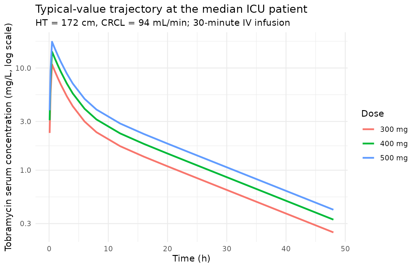
Concentration-time VPC (analogue of Figures 1 and 4)
# Replicates the spread analogous to Conil 2010 Figure 1 (individual
# observed concentrations) and Figure 4 / Table 3 (Monte Carlo simulated
# concentrations across doses). Median and 90% prediction interval per
# dose level.
sim_stoch |>
  filter(time > 0) |>
  group_by(treatment, time) |>
  summarise(
    Q05 = quantile(Cc, 0.05, na.rm = TRUE),
    Q50 = quantile(Cc, 0.50, na.rm = TRUE),
    Q95 = quantile(Cc, 0.95, na.rm = TRUE),
    .groups = "drop"
  ) |>
  ggplot(aes(time, Q50, colour = treatment, fill = treatment)) +
  geom_ribbon(aes(ymin = Q05, ymax = Q95), alpha = 0.20, colour = NA) +
  geom_line(linewidth = 0.9) +
  scale_y_log10() +
  labs(
    x = "Time (h)",
    y = "Tobramycin serum concentration (mg/L, log scale)",
    colour = "Dose", fill = "Dose",
    title    = "VPC by dose for the typical ICU patient",
    subtitle = paste0(
      "Median and 90% prediction interval; ", n_per_dose,
      " Monte Carlo subjects per dose"
    )
  ) +
  theme_minimal()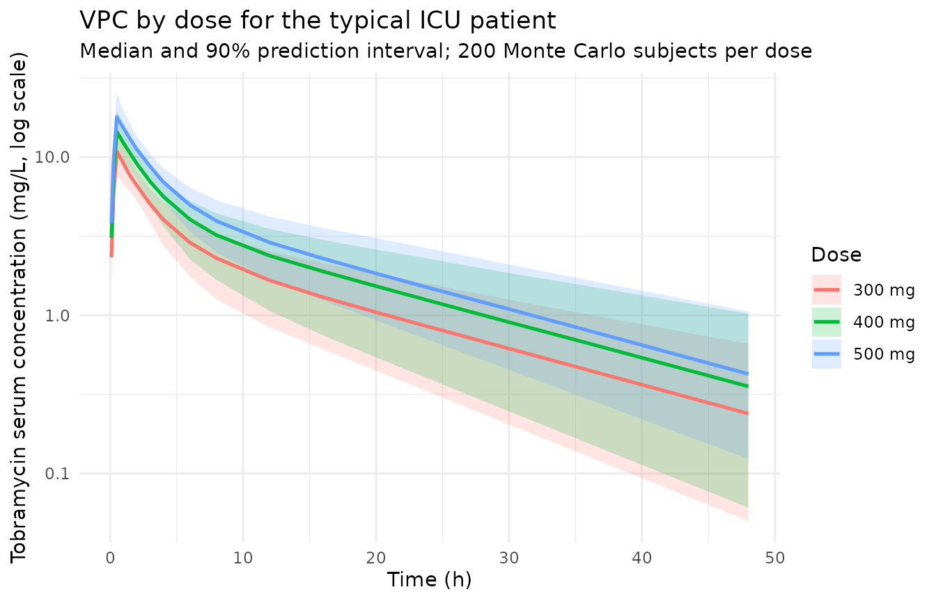
PKNCA validation
PKNCA computes Cmax, AUC0-inf, and terminal half-life per subject per dose level. The treatment grouping variable carries the dose level through to the comparison.
sim_for_nca <- sim_stoch |>
  dplyr::filter(!is.na(Cc)) |>
  dplyr::select(id, time, Cc, treatment) |>
  as.data.frame()

# Defensive time = 0 row per (id, treatment); for IV-bolus / IV-infusion
# models pre-dose Cc = 0 is the correct value.
sim_for_nca <- dplyr::bind_rows(
  sim_for_nca,
  sim_for_nca |> dplyr::distinct(id, treatment) |>
    dplyr::mutate(time = 0, Cc = 0)
) |>
  dplyr::distinct(id, treatment, time, .keep_all = TRUE) |>
  dplyr::arrange(id, treatment, time)

dose_for_nca <- events |>
  dplyr::filter(evid == 1L) |>
  dplyr::select(id, time, amt, treatment) |>
  as.data.frame()

conc_obj <- PKNCA::PKNCAconc(
  data    = sim_for_nca,
  formula = Cc ~ time | treatment + id,
  concu   = "mg/L",
  timeu   = "hr"
)
dose_obj <- PKNCA::PKNCAdose(
  data    = dose_for_nca,
  formula = amt ~ time | treatment + id,
  doseu   = "mg"
)

intervals <- data.frame(
  start      = 0,
  end        = Inf,
  cmax       = TRUE,
  tmax       = TRUE,
  aucinf.obs = TRUE,
  half.life  = TRUE
)

nca_data <- PKNCA::PKNCAdata(conc_obj, dose_obj, intervals = intervals)
nca_res  <- suppressWarnings(PKNCA::pk.nca(nca_data))
Trough at 24 h and Peak at 1 h (paper protocol-specific timepoints)
Conil 2010 reports two protocol-specific concentrations in Table 3: “Peak” (sampled 30 minutes after the end of the 30-minute infusion, i.e. at t = 1 h) and “C24h” (concentration at t = 24 h). These are distinct from a standard NCA Cmax, which here falls at the end of infusion (t = 0.5 h) where the concentration is slightly higher than at 1 h. The Peak and C24h summaries are computed by direct extraction from the simulated profiles.
protocol_concs <- sim_stoch |>
  dplyr::filter(time %in% c(1.0, 24.0)) |>
  dplyr::mutate(
    metric = dplyr::case_when(
      time == 1.0  ~ "Peak (t = 1 h)",
      time == 24.0 ~ "C24h (t = 24 h)"
    )
  ) |>
  dplyr::group_by(treatment, metric) |>
  dplyr::summarise(
    Simulated_mean = mean(Cc, na.rm = TRUE),
    Simulated_sd   = sd(Cc, na.rm = TRUE),
    .groups = "drop"
  )

published_protocol <- tibble::tribble(
  ~treatment, ~metric,             ~Reference_mean, ~Reference_sd,
  "300 mg",   "Peak (t = 1 h)",    9.01,            2.64,
  "300 mg",   "C24h (t = 24 h)",   0.96,            0.48,
  "400 mg",   "Peak (t = 1 h)",    12.01,           3.52,
  "400 mg",   "C24h (t = 24 h)",   1.28,            0.64,
  "500 mg",   "Peak (t = 1 h)",    15.01,           4.41,
  "500 mg",   "C24h (t = 24 h)",   1.60,            0.81
)

protocol_cmp <- published_protocol |>
  dplyr::inner_join(protocol_concs, by = c("treatment", "metric")) |>
  dplyr::mutate(
    Reference = sprintf("%.2f +/- %.2f", Reference_mean, Reference_sd),
    Simulated = sprintf("%.2f +/- %.2f", Simulated_mean, Simulated_sd),
    `% diff (mean)` = sprintf(
      "%+.1f%%",
      (Simulated_mean - Reference_mean) / Reference_mean * 100
    )
  ) |>
  dplyr::select(treatment, metric, Reference, Simulated, `% diff (mean)`)

knitr::kable(
  protocol_cmp,
  caption = paste0(
    "Simulated vs Conil 2010 Table 3 protocol-specific concentrations ",
    "(mean +/- SD, mg/L). Typical-covariate patient (HT = 172 cm, ",
    "CRCL = 94 mL/min); 1000 Monte Carlo simulations in the paper, ",
    n_per_dose, " here per dose."
  ),
  align = c("l", "l", "r", "r", "r")
)| treatment | metric | Reference | Simulated | % diff (mean) |
|---|---|---|---|---|
| 300 mg | Peak (t = 1 h) | 9.01 +/- 2.64 | 9.20 +/- 1.55 | +2.1% |
| 300 mg | C24h (t = 24 h) | 0.96 +/- 0.48 | 0.91 +/- 0.40 | -5.1% |
| 400 mg | Peak (t = 1 h) | 12.01 +/- 3.52 | 12.45 +/- 2.14 | +3.7% |
| 400 mg | C24h (t = 24 h) | 1.28 +/- 0.64 | 1.29 +/- 0.60 | +0.7% |
| 500 mg | Peak (t = 1 h) | 15.01 +/- 4.41 | 15.41 +/- 2.41 | +2.7% |
| 500 mg | C24h (t = 24 h) | 1.60 +/- 0.81 | 1.58 +/- 0.64 | -1.1% |
Comparison against published NCA
Conil 2010 Table 3 reports a Monte Carlo AUC for each dose. The
ncaComparisonTable below sets the simulated Cmax (true maximum, at end
of infusion) and AUC0-inf side-by-side with the paper’s Peak and AUC
values. The paper’s Peak is the concentration at t = 1 h (sampling
convention), which is below the true Cmax at t = 0.5 h, so the Cmax row
is expected to read slightly higher than the paper’s Peak (a positive %
diff on the order of 10-15 percent); the AUC0-inf row should match
Conil’s AUC closely because tobramycin’s two-compartment disposition is
captured to t = Inf by both PKNCA and the paper’s 1000-replicate
simulation. Discrepancies > 20% are flagged with *.
published_nca <- tibble::tribble(
  ~treatment, ~cmax,  ~aucinf.obs,
  "300 mg",   9.01,    82,
  "400 mg",   12.01,   109,
  "500 mg",   15.01,   137
)

cmp <- nlmixr2lib::ncaComparisonTable(
  simulated     = nca_res,
  reference     = published_nca,
  by            = "treatment",
  units         = c(cmax = "mg/L", aucinf.obs = "mg*h/L"),
  tolerance_pct = 20
)

knitr::kable(
  cmp,
  caption = paste0(
    "Simulated vs Conil 2010 Table 3 NCA-style summaries for the ",
    "typical ICU patient. * = differs from reference by more than ",
    "+/- 20%."
  ),
  align = c("l", "l", "r", "r", "r")
)| NCA parameter | treatment | Reference | Simulated | % diff |
|---|---|---|---|---|
| Cmax (mg/L) | 300 mg | 9.01 | 10.9 | +21.0%* |
| Cmax (mg/L) | 400 mg | 12 | 14.5 | +20.5%* |
| Cmax (mg/L) | 500 mg | 15 | 17.9 | +19.4% |
| AUC0-∞ (obs) (mg*h/L) | 300 mg | 82 | 76.2 | -7.0% |
| AUC0-∞ (obs) (mg*h/L) | 400 mg | 109 | 110 | +0.6% |
| AUC0-∞ (obs) (mg*h/L) | 500 mg | 137 | 132 | -3.4% |
Assumptions and deviations
CL covariate equation – linear-additive deviation form, NOT power or divisive normalization. Conil 2010 Table 2 reports the typical CL as
TVCL = THETA(1) + THETA(2) * (COCK - 94) + THETA(3) * (HEIG - 172), with THETA(1) = 3.83 L/h, THETA(2) = 0.020 L/h per mL/min, THETA(3) = 0.052 L/h per cm. This is a linear-additive deviation from the population reference covariates 94 mL/min and 172 cm. The packaged model encodes the equation verbatim:cl <- (exp(lcl) + e_crcl_cl * (CRCL - 94) + e_ht_cl * (HT - 172)) * exp(etalcl), withlcl = log(3.83)so thatexp(lcl)recovers the 3.83 L/h intercept. The exponential IIV multiplierexp(etalcl)is applied outside the additive covariate term, matching the paper’sCL = TVCL * EXP(ETA(1))form (Conil 2010 Table 2 equation block).Q and V2 carry no IIV in the final model. Table 2 reports Omega 3 (Q) and Omega 4 (V2) as “Fixed” in the intermediate and final models. The paper’s Methods explain that the inter-individual variability of Q was “very low” and that V2’s Omega in the basic model was unreliable (
287% precision); both were therefore fixed to zero. The packaged model includes noetalqoretalvpparameter, leaving Q and V2 as typical-value-only parameters.Residual error – proportional, encoded as
sqrt(0.055). Table 2 reports Sigma 1 = 0.055 for the final model under the NONMEM conventionY = F * (1 + EPS(1))with EPS ~ N(0, SIGMA). 0.055 is the variance of EPS, so the proportional-error SD issqrt(0.055)~= 0.234 (CV 23%); this is whatpropSdrepresents in nlmixr2’s~ prop(propSd)form.CRCLsource column isCOCK(raw Cockcroft-Gault, not BSA-normalized). The canonicalCRCLcolumn ininst/references/covariate-columns.mdaccepts raw Cockcroft-Gault mL/min as one valid form; precedent isDelattre_2010_amikacin.R, another aminoglycoside ICU model with the same source-assay convention. The per-modelcovariateData[[CRCL]]$units = "mL/min"andnotesfield document the raw / non-BSA-normalized status. Reference 94 mL/min (population median, Conil 2010 Methods “Simulation and dosage regimen propositions”) is paper-derived; do NOT compare the magnitude ofe_crcl_cl = 0.020 L/h per mL/minagainst the BSA-normalized reference values (80, 90, or 100 mL/min/1.73 m^2) listed in the canonical entry – the units differ.HTsource column isHEIG. The canonicalHTcolumn ininst/references/covariate-columns.mdalready records the Naik 2016, Zhang 2018, and Angeli 2016 precedents for linear-additive centered effects. Reference 172 cm matches Conil 2010 Methods “Simulation and dosage regimen propositions”. Height was retained in the final model in preference to body weight because, as discussed in Conil 2010 Discussion, ICU patients often present with oedema that biases total body weight; height correlated more strongly with CL than TBW or IBW in the stepwise analysis.Peak vs Cmax – sampling-time convention. Conil 2010 Table 3 “Peak” is sampled 30 minutes after the end of the 30-minute infusion, i.e. at t = 1 h. PKNCA’s
cmaxis the maximum observed concentration on the sampling grid, which for a two-compartment IV-infusion model is at the end of infusion (t = 0.5 h, where central-compartment concentration peaks before alpha-phase distribution to the peripheral compartment). The packaged simulation samples both times. The “NCA comparison” table compares PKNCA Cmax against the paper’s Peak (expect a positive bias of ~10-15% because Cmax > C(1 h)); the protocol-specific table compares the simulated concentration at t = 1 h directly against the paper’s Peak. Both checks should be considered together.Cohort covariates fixed at the typical-patient values. Conil 2010 Table 3 Monte Carlo simulations are themselves performed at HT = 172 cm and CRCL = 94 mL/min with IIV draws only; the virtual cohort here mirrors that convention so the comparison is like-for-like. A broader virtual cohort with covariates drawn from the Table 1 distributions would simulate the full ICU population rather than the typical patient and is outside the scope of this validation.
Number of Monte Carlo replicates. Conil 2010 performed 1000 replicates per dose. The vignette uses 200 replicates per dose to keep the render time well under the 5-minute pkgdown budget. The reduced sample size widens the simulated SD but does not bias the simulated mean; mean comparisons should track Table 3 closely.
Race / ethnicity not modeled. Conil 2010 does not report race composition. The single-centre French ICU cohort is presumed predominantly European but race was not tested as a covariate; no race effect is included in the model.
Concentration units. The model uses
mg/L(paper convention for tobramycin). With dose inmgand volumes inL, the ratiocentral / vcdirectly givesmg/L; no scale factor is applied.Single-dose simulation. The vignette simulates one 30-minute IV infusion per subject because Table 3 reports the single-dose Monte Carlo simulation Conil 2010 used to formulate dosing recommendations. The paper’s clinical regimen is 5 mg/kg once daily for 3-5 days; with a terminal half-life ~10 h, the single-dose AUC0-inf is the relevant exposure for the once-daily target (24 h dose interval ~= 2.4 half-lives, so accumulation is modest).
No erratum on file. A search for published corrections to Conil 2010 in the British Journal of Clinical Pharmacology did not surface a corrigendum. Should one appear later, the parameter values here would need to be revisited.