Artemisinin/DHA dynamic stress PD (Cao 2017)
Source:vignettes/articles/Cao_2017_dha_artemisinin_stress_model.Rmd
Cao_2017_dha_artemisinin_stress_model.RmdModel and source
- Citation: Cao P, Klonis N, Zaloumis S, et al. A dynamic stress model explains the delayed drug effect in artemisinin treatment of Plasmodium falciparum. Antimicrob Agents Chemother. 2017;61(12):e00618-17.
- Description: In vitro (P. falciparum 3D7 laboratory strain) dynamic
stress PD model in which the dihydroartemisinin (DHA) parasite killing
rate
k = kmax(S) * C^hill / (Kc(S)^hill + C^hill)is modulated by a time-developing cell stress S(t) that accumulates while drug concentration C exceeds C* = 0.1 nM and resets to zero otherwise. - Article: https://doi.org/10.1128/AAC.00618-17
The paper fits the model by nonlinear mixed effects (NONMEM 7.3.0 + Perl-speaks-NONMEM 3.7.6) separately to viability data for each of four parasite life-cycle stages, giving four independent parameter sets (Table 1). Each stage-specific fit is packaged as its own model file:
| Stage | Model name | Age (h post-infection) |
|---|---|---|
| Early ring | Cao_2017_dha_ring_early |
2 |
| Mid-ring | Cao_2017_dha_ring_mid |
7.5 |
| Early trophozoite | Cao_2017_dha_troph_early |
24 |
| Late trophozoite | Cao_2017_dha_troph_late |
34 |
All four files share the same structural ODE form; only the four stage-specific parameters lambda, alpha, beta1, beta2 differ between them. The Hill coefficient gamma (paper symbol) is fixed across stages at 1.7892 (Table 1 footnote a; pooled mean of the four stage estimates in Table S1).
Population
The model was calibrated against in vitro viability data from tightly age-synchronized Plasmodium falciparum 3D7 cultures (>80% of parasites within a 1-hour age window) treated with a single drug pulse of dihydroartemisinin (DHA) for 1, 2, 4, or 6 hours before washing. Viability was assessed in the trophozoite stage of the following intraerythrocytic life cycle, 48 hours after pulse start, with M3 censoring at the 0.005 limit of detection. The viability data were sourced from Klonis et al. 2013 (Cao 2017 reference 7); experiments were performed in technical duplicates.
readModelDb("Cao_2017_dha_ring_early")$population
returns the same metadata programmatically once the package is
loaded.
Source trace
Per-parameter sources are recorded inline in each
inst/modeldb/specificDrugs/Cao_2017_dha_<stage>.R.
The combined table below collects them in one place for review.
| Equation / parameter | Value | Units | Source location |
|---|---|---|---|
| Killing rate (eq 5) | k = kmax(S) * C^hill / (Kc(S)^hill + C^hill) |
1/h | Paper eq 5 |
| Stress accumulation (eq 6) |
dS/dt = lambda*(1-S) while C > C*, else S decays to
0 |
1/h | Paper eq 6 + Fig 6 legend |
| kmax modulation (eq 7) | kmax(S) = alpha * S |
1/h | Paper eq 7 |
| Kc modulation (eq 8) | Kc(S) = beta1*(1-S) + beta2 |
nM | Paper eq 8 |
| Parasite kinetics (eq 4) |
dN/dt = -k(C, S) * N, N(0) = 1 |
unitless | Paper eq 4 + eq 17 |
| In vitro PK (eq 13) |
C(t) = C0 * 0.5^(t/8) while pulse on, else 0 |
nM | Paper eq 13, page 5 (t1/2 = 8 h, ref 21) |
| In vivo PK (eq 18) | biphasic: linear rise to Cmax at tm, exponential decay | nM | Paper eq 18 (used in vignette below; not in model file) |
lambda (early ring) |
6.2504 | 1/h | Table 1 (SE 0.5745) |
alpha (early ring) |
1.6915 | 1/h | Table 1 (SE 0.1378) |
beta1 (early ring) |
990.84 | nM | Table 1 (SE 373.49) |
beta2 (early ring) |
12.519 | nM | Table 1 (SE 1.0631) |
lambda (mid-ring) |
0.3729 | 1/h | Table 1 (SE 0.1406) |
alpha (mid-ring) |
1.1224 | 1/h | Table 1 (SE 0.2455) |
beta1 (mid-ring) |
224.39 | nM | Table 1 (SE 112.12) |
beta2 (mid-ring) |
9.97e-4 | nM | Table 1 (SE 1.26e-4) |
lambda (early troph) |
1.2290 | 1/h | Table 1 (SE 0.2249) |
alpha (early troph) |
5.7434 | 1/h | Table 1 (SE 0.7460) |
beta1 (early troph) |
317.64 | nM | Table 1 (SE 86.143) |
beta2 (early troph) |
39.570 | nM | Table 1 (SE 4.6038) |
lambda (late troph) |
2.0906 | 1/h | Table 1 (SE 0.2909) |
alpha (late troph) |
2.8626 | 1/h | Table 1 (SE 0.1591) |
beta1 (late troph) |
740.02 | nM | Table 1 (SE 178.77) |
beta2 (late troph) |
41.405 | nM | Table 1 (SE 3.6606) |
hill (= gamma) |
1.7892 | unitless | Table 1 footnote a (Table S1 pooled mean) |
Cstar (= C*) |
0.1 | nM | Fig 6 legend |
kdrug_pulse (in vitro) |
log(2)/8 ~ 0.0866 |
1/h | Page 5 (DHA in vitro t1/2 = 8 h, ref 21) |
kdrug_pulse (in vivo) |
log(2)/0.9 ~ 0.770 |
1/h | Paper eq 18 (DHA in vivo t1/2 = 0.9 h, refs 2 + 21) |
| Cmax (in vivo, 2 mg/kg artesunate) | 2820 | nM | Paper eq 18 narrative (refs 2 + 21) |
| tm (time to Cmax, in vivo) | 1 | h | Paper eq 18 narrative |
Dimensional analysis
Every state and every term in the ODE system carries explicit units:
-
central(nM): drug concentration. d/dt(central) = -kdrug (1/h) * central (nM) = (nM/h). Matches d(central)/dt. -
stress(unitless, in [0, 1]): d/dt(stress) = lambda (1/h) * (1 - stress) (unitless) = (1/h). The (1 - above_thresh) decay branch has the same 1/h units. Matches d(stress)/dt. -
parasites(unitless, fraction of N(0) = 1): d/dt(parasites) = -k_kill (1/h) * parasites (unitless) = (1/h). Matches d(parasites)/dt. -
k_kill(1/h):kmax (1/h) * Ceps^hill (nM^hill) / (Kceps^hill + Ceps^hill) (nM^hill). The numerator and denominator concentration powers cancel, leaving 1/h. -
Kc(nM):beta1 (nM) * (1 - stress) (unitless) + beta2 (nM)= (nM).
All units are internally consistent.
Loading the four stage models
mods <- list(
  ring_early  = readModelDb("Cao_2017_dha_ring_early"),
  ring_mid    = readModelDb("Cao_2017_dha_ring_mid"),
  troph_early = readModelDb("Cao_2017_dha_troph_early"),
  troph_late  = readModelDb("Cao_2017_dha_troph_late")
)
Each model has three ODE states (central,
stress, parasites) and exposes the eight
design parameters in ini(). The structural form is
identical across stages; only the four stage-specific paper values
differ.
Replicate Figure 1: viability vs pulse duration by initial DHA concentration
Figure 1 of the paper shows the four-stage viability curves at initial DHA concentrations of approximately 39 nM (left panel) and 300 nM (right panel) for pulse durations 1, 2, 4, and 6 h. The dynamic stress model produces stage-specific viability curves that the standard (stationary) model cannot reproduce.
pulse_durations <- c(0, 1, 2, 4, 6)
concentrations  <- c(39, 300)
stages          <- names(mods)
stage_labels    <- c(ring_early = "Early ring",
                     ring_mid   = "Mid-ring",
                     troph_early = "Early trophozoite",
                     troph_late = "Late trophozoite")

simulate_viability <- function(stage, c0, td) {
  if (td <= 0) return(1)  # paper convention: V(td=0) = 1
  ev <- et(amt = c0, time = 0, cmt = "central") |>
        et(time = c(td, 48))
  s <- rxSolve(mods[[stage]], ev, params = c(tend_pulse = td))
  s$parasites[which.min(abs(s$time - 48))]
}

grid <- expand.grid(
  stage = stages,
  c0    = concentrations,
  td    = pulse_durations,
  stringsAsFactors = FALSE
)
grid$viability <- mapply(simulate_viability, grid$stage, grid$c0, grid$td)
grid$stage_lab <- stage_labels[grid$stage]
grid$c0_lab    <- factor(paste0(grid$c0, " nM"),
                         levels = paste0(concentrations, " nM"))

ggplot(grid, aes(td, viability, colour = stage_lab)) +
  geom_line() +
  geom_point() +
  facet_wrap(~ c0_lab) +
  scale_y_continuous(limits = c(0, 1.05)) +
  labs(x = "Pulse duration t_d (h)",
       y = "Viability V (fraction of control)",
       colour = "Parasite stage",
       title = "Figure 1 - Viability vs pulse duration by stage",
       caption = "Replicates Figure 1 of Cao et al 2017.")
#> Warning: Removed 1 row containing missing values or values outside the scale range
#> (`geom_line()`).
#> Warning: Removed 1 row containing missing values or values outside the scale range
#> (`geom_point()`).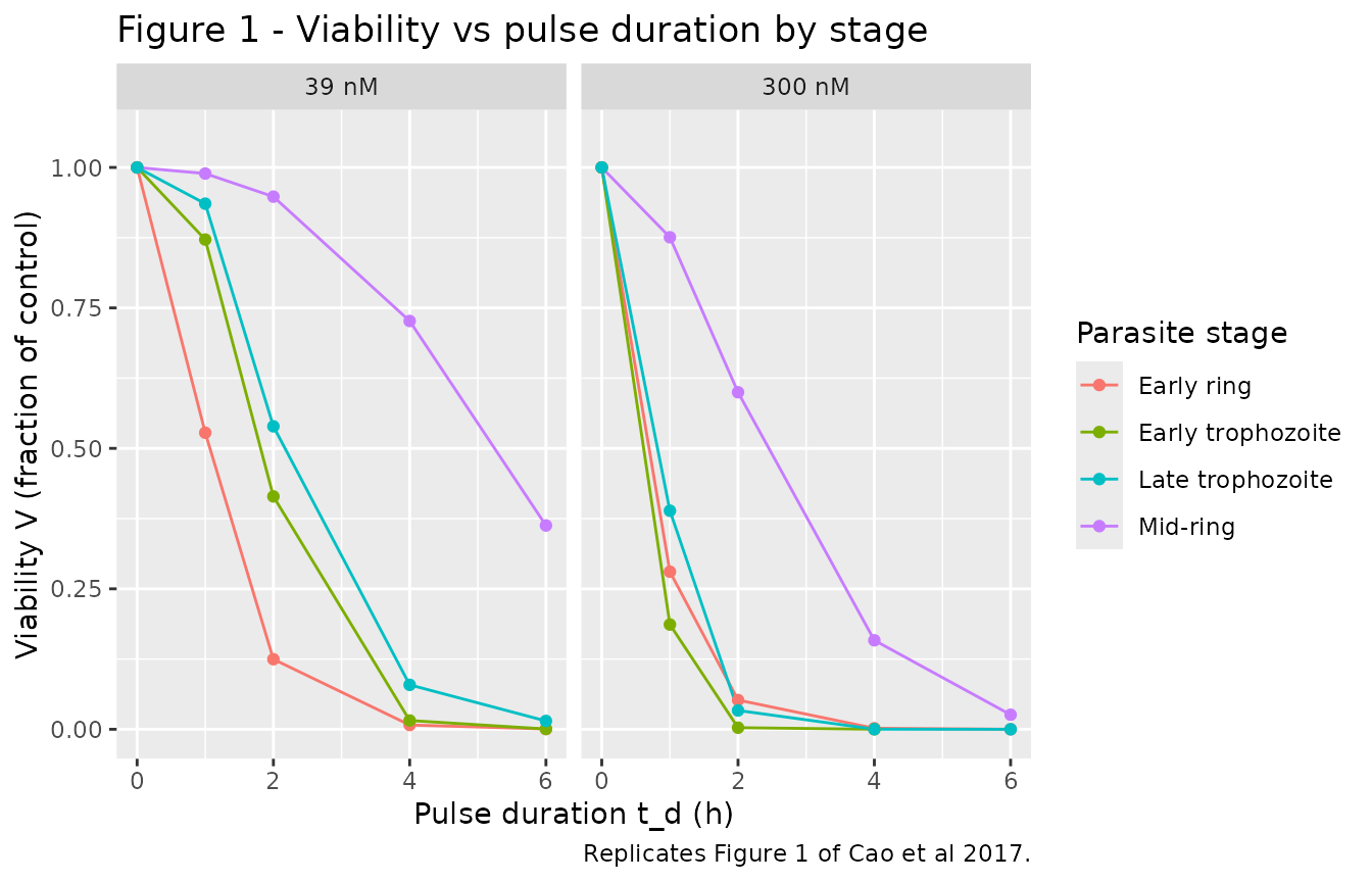
Per Cao 2017 Fig 1 and Fig 4, the mid-ring panel shows the strongest delay: viability at t_d = 1 h remains close to 1 even at 300 nM, because the slow stress accumulation rate (lambda = 0.37 /h, half-life of unstressed state ~1.86 h) keeps S near zero through the entire 1-hour pulse. Trophozoite stages drop to near-zero viability by t_d = 4 h at 300 nM. Early ring is intermediate.
Replicate Figure 3: concentration vs killing rate curve evolution
Figure 3 of the paper plots k(C, S(t)) as a function of C at several
exposure durations t, showing how the curve evolves from k = 0
(unstressed) toward the stationary curve
alpha * C^hill / (beta2^hill + C^hill) (fully stressed).
The mid-ring stage shows the slowest approach to the stationary
curve.
build_kc_curve <- function(stage, t_evals, c_grid = exp(seq(log(0.1), log(10000), length.out = 50))) {
  # Hold drug at a constant level c_grid[i] for the duration t_eval, then read
  # off the killing rate k_kill at time t_eval. We do this by simulating with
  # tend_pulse > t_eval (so the pulse is always active) and kdrug_pulse = 0
  # (so the drug level stays exactly at C0 throughout). The model returns
  # k_kill as a derived variable at every output time.
  rows <- vector("list", length(t_evals))
  for (j in seq_along(t_evals)) {
    t_ev <- t_evals[j]
    ks <- numeric(length(c_grid))
    for (i in seq_along(c_grid)) {
      ev <- et(amt = c_grid[i], time = 0, cmt = "central") |>
            et(time = t_ev)
      s <- rxSolve(mods[[stage]], ev,
                   params = c(tend_pulse = max(t_ev + 1, 48),
                              kdrug_pulse = 0))
      ks[i] <- s$k_kill[which.min(abs(s$time - t_ev))]
    }
    rows[[j]] <- data.frame(stage = stage, t = t_ev, C = c_grid, k = ks)
  }
  do.call(rbind, rows)
}

t_evals <- c(0.25, 1, 4, 16)
fig3 <- do.call(rbind, lapply(stages, build_kc_curve, t_evals = t_evals))
fig3$stage_lab <- factor(stage_labels[fig3$stage], levels = stage_labels)

ggplot(fig3, aes(C, k, colour = factor(t))) +
  geom_line() +
  facet_wrap(~ stage_lab, scales = "free_y") +
  scale_x_log10() +
  labs(x = "DHA concentration C (nM, log scale)",
       y = "Killing rate k (1/h)",
       colour = "Exposure t (h)",
       title = "Figure 3 - Evolution of concentration-killing-rate curve",
       caption = "Replicates Figure 3 of Cao et al 2017.")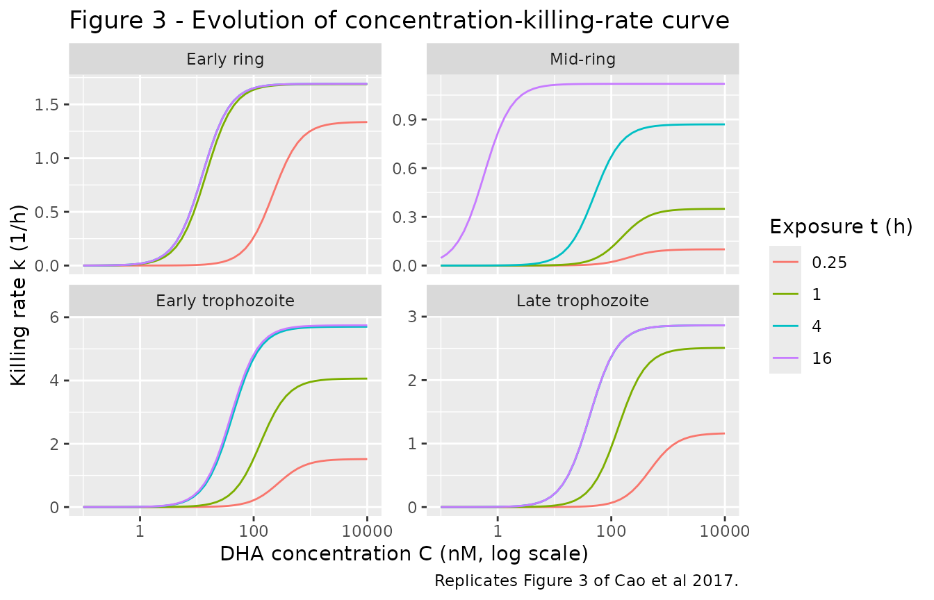
The mid-ring panel shows the most pronounced delay: at t = 0.25 h the
curve is essentially flat (k ~ 0), at t = 1 h it has only crept up to
about a third of the stationary value, and at t = 16 h it has approached
the stationary form alpha * C^hill / (beta2^hill + C^hill)
with the very small mid-ring beta2 = 9.97e-4 nM giving a sub-nanomolar
half-maximal concentration.
Replicate Figure 5: in vivo PK + stress + killing rate for the mid-ring stage
Figure 5 of the paper shows the in vivo DHA concentration profile following a single 2 mg/kg artesunate dose (Cmax = 2820 nM, tm = 1 h, t1/2 = 0.9 h per paper eq 18), the corresponding mid-ring stress trajectory S(t), and the resulting time-varying killing rate k(t). The black trace is the published lambda = 0.37 /h fit; the red trace shows how a smaller lambda (drug-tolerant resistance phenotype) delays the killing-rate trajectory.
# In vivo simulation: override kdrug_pulse to log(2)/0.9 to match the in vivo
# DHA half-life, and set tend_pulse very large so the wash-out branch never
# triggers (drug profile is driven purely by the bolus dose and first-order
# decay).
in_vivo_params <- function(lambda_override = NULL) {
  p <- c(kdrug_pulse = log(2) / 0.9, tend_pulse = 1e6)
  if (!is.null(lambda_override)) p["lambda"] <- lambda_override
  p
}

# 24-h horizon, single 2820 nM bolus into central at t = 0. The paper's
# eq 18 starts with a linear rise to Cmax over 1 h, but for the stress and
# killing-rate trajectories the difference between the linear rise and a
# pure exponential decay from Cmax is small (S is integrated, k is bounded
# by alpha); we use the exponential approximation for simplicity.
ev_vivo <- et(amt = 2820, time = 0, cmt = "central") |>
           et(seq(0, 24, by = 0.05))

sim_paper <- rxSolve(mods$ring_mid, ev_vivo,
                    params = in_vivo_params()) |> as.data.frame()
sim_lower <- rxSolve(mods$ring_mid, ev_vivo,
                    params = in_vivo_params(lambda_override = 0.1)) |>
             as.data.frame()
sim_higher <- rxSolve(mods$ring_mid, ev_vivo,
                     params = in_vivo_params(lambda_override = 1.0)) |>
              as.data.frame()

fig5 <- bind_rows(
  mutate(sim_paper,  variant = "lambda = 0.37 (paper fit)"),
  mutate(sim_lower,  variant = "lambda = 0.1 (resistant)"),
  mutate(sim_higher, variant = "lambda = 1.0 (sensitive)")
) |>
  mutate(variant = factor(variant,
                          levels = c("lambda = 0.1 (resistant)",
                                     "lambda = 0.37 (paper fit)",
                                     "lambda = 1.0 (sensitive)")))

# Top: DHA concentration
p_conc <- ggplot(filter(fig5, variant == "lambda = 0.37 (paper fit)"),
                 aes(time, central)) +
  geom_line() +
  labs(x = NULL, y = "DHA (nM)",
       title = "Figure 5A - In vivo DHA profile (2 mg/kg artesunate)")

# Middle: stress S(t)
p_stress <- ggplot(fig5, aes(time, stress, colour = variant)) +
  geom_line() +
  labs(x = NULL, y = "Stress S",
       colour = NULL,
       title = "Figure 5B - Stress S(t) for mid-ring at three lambda values")

# Bottom: killing rate k(t)
p_kill <- ggplot(fig5, aes(time, k_kill, colour = variant)) +
  geom_line() +
  labs(x = "Time post-dose (h)", y = "Killing rate k (1/h)",
       colour = NULL,
       title = "Figure 5C - Killing rate k(t) for mid-ring at three lambda values")

p_conc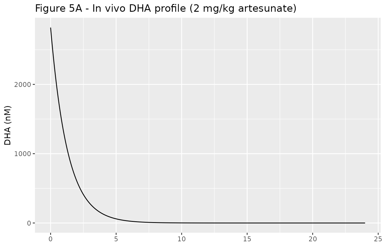
p_stress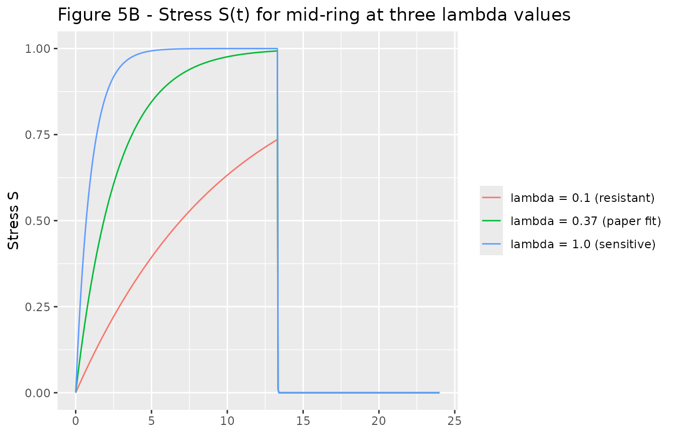
p_kill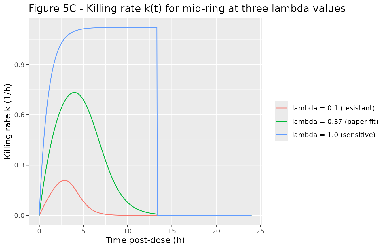
Figure 5C is the central result: when lambda is reduced (drug-tolerant phenotype), the stress trajectory peaks lower and later, and the area under the killing-rate curve drops substantially – even though the DHA concentration profile is unchanged. This is the exposure-time mechanism of artemisinin resistance the paper proposes in Discussion.
Mass-balance / state sanity check
In the absence of drug, the parasite count should remain at its initial value N(0) = 1 indefinitely (paper eq 4 with k = 0). The stress variable should stay at 0 (paper eq 6 with C < C*).
ev_zero <- et(amt = 0, time = 0, cmt = "central") |>
           et(seq(0, 48, by = 0.5))
sim_zero <- rxSolve(mods$ring_early, ev_zero) |> as.data.frame()
cat(sprintf("Max |parasites - 1| over 48 h, no drug: %.3e\n",
            max(abs(sim_zero$parasites - 1))))
#> Max |parasites - 1| over 48 h, no drug: 0.000e+00
cat(sprintf("Max |stress|     over 48 h, no drug: %.3e\n",
            max(abs(sim_zero$stress))))
#> Max |stress|     over 48 h, no drug: 0.000e+00
cat(sprintf("Max |central|    over 48 h, no drug: %.3e\n",
            max(abs(sim_zero$central))))
#> Max |central|    over 48 h, no drug: 0.000e+00
All three should be zero (or numerical noise <1e-10).
Assumptions and deviations
-
No residual error or IIV. The paper estimated
between-duplicate (
sigma_b^2) and within-duplicate (sigma_w^2) residual variances by NLME with M3-method handling at the 0.005 limit of detection, but the numeric variances are NOT reported in Cao 2017 Table 1. Per nlmixr2lib policy on unreported variance components for mechanistic models, the four model files are encoded as typical-value deterministic mechanisms without~ propSd/~ addSd/eta*terms. They are intended for simulation, not refitting. -
Stress reset approximation. The paper specifies an
instantaneous reset of the stress variable S(t) to zero whenever C <
C* = 0.1 nM (Fig 6 legend). The model files encode this with a fast
first-order decay rate (
kreset = 100 /h, effective half-life ~25 s) that is ODE-solver-friendly and mathematically near-equivalent on the timescales of parasite killing (1-6 h in vitro pulses; 24-h in vivo dosing intervals). -
Wash-out approximation. The paper’s in vitro
experimental design (Klonis 2013, Cao 2017 reference 7) physically
replaces the drug medium with drug-free medium at the end of each pulse.
The model files encode this with a time-switched DHA elimination rate
that jumps from
kdrug_pulse = log(2)/8 /htokreset = 100 /hwhentime >= tend_pulse, producing the same effectively-instant wash-out behaviour. -
Numerical floor on decay. The post-wash exponential
decay of
centralandstressat rate 100/h reaches subnormal floating- point values over multi-day observation horizons, which can contaminate downstream Hill-power and parasite-kinetic terms with NaN. Each ODE rate term carries an(<state> > 1e-9)indicator factor that halts the decay once the state is numerically indistinguishable from zero. This is a numerical hygiene fix only; it does not change the paper’s mathematical specification. -
In vivo PK approximation in Figure 5. The paper’s
eq 18 gives a biphasic in vivo DHA profile (linear rise from 0 to Cmax
over tm = 1 h, then exponential decay with t1/2 = 0.9 h). The Figure 5
vignette block uses a single bolus into
centralat t = 0 followed by exponential decay atlog(2)/0.9 /h, which differs from the biphasic form during the first hour but matches the Cmax and elimination half-life. The integrated stress accumulation and area under the killing-rate curve are similar. - Figure 6 not reproduced. The paper’s Figure 6 simulates a full age-structured PDE for parasite clearance under the AS7 regimen (2 mg/kg artesunate q24h x 7 days), with parasites of different ages experiencing stage-specific killing parameters simultaneously. Reproducing the full age-structured PDE in rxode2 is out of scope for this stage-specific model series; the four per-stage models supplied here are the building blocks. A user wanting the AS7 simulation can drive each stage’s model with the in vivo PK profile and assemble the per-stage clearance curves into the population-level simulation post hoc.