Venlafaxine and O-desmethylvenlafaxine (Wang 2022)
Source:vignettes/articles/Wang_2022_venlafaxine.Rmd
Wang_2022_venlafaxine.RmdModel and source
- Citation: Wang Z, Li L, Huang S, Wang X, Liu S, Li X, Kong W, Ni X, Zhang M, Huang S, Tan Y, Wen Y, Shang D. Joint population pharmacokinetic modeling of venlafaxine and O-desmethyl venlafaxine in healthy volunteers and patients to evaluate the impact of morbidity and concomitant medication. Front Pharmacol. 2022;13:978202. doi:10.3389/fphar.2022.978202
- Description: Joint parent-metabolite population PK model for oral venlafaxine (VEN) and its active metabolite O-desmethylvenlafaxine (ODV, desvenlafaxine) in Chinese healthy male volunteers and psychiatric patients (Wang 2022). One-compartment disposition for each analyte with first-order absorption (ka fixed at 0.63 1/h). The absorbed dose splits at absorption: a fraction fm_odv is converted pre-systemically (first pass) and enters the ODV compartment directly, and the remainder enters the VEN compartment. All systemic VEN clearance forms ODV (k23 = CL/V), and ODV is cleared with CL_odv. Clearances and volumes are apparent (relative to the unknown oral bioavailability). The model works on a MOLAR basis: doses are in umol of venlafaxine and both concentrations are in umol/L, as in the source figures. Patient status lowers VEN CL/F by 61.7 percent relative to healthy volunteers; concomitant amisulpride lowers VEN CL/F by 39.2 percent and raises ODV CL/F by 59.3 percent. Proportional residual error on each analyte.
- Article: https://doi.org/10.3389/fphar.2022.978202 (open access)
Wang et al. fitted venlafaxine (VEN) and its active metabolite
O-desmethylvenlafaxine (ODV) jointly in NONMEM 7.3 (FOCEI, ADVAN6). A
dose enters a single absorption depot (ka fixed at 0.63 1/h). A fraction
FP of the absorbed dose is converted to ODV before it reaches the
circulation and enters the ODV compartment directly; the rest enters the
VEN compartment. All systemic VEN elimination forms ODV (Figure 1:
K23 is the only exit from the VEN compartment), and ODV is
eliminated by K30.
Molar units. The source figures plot both analytes
in umol/L, so the model works in moles: doses are entered in umol of
venlafaxine and Cc (VEN) and Cc_odv (ODV) are
returned in umol/L. Molar amounts also make the VEN-to-ODV conversion
stoichiometric. The constants below convert doses and
concentrations.
mw_ven <- 277.40 # g/mol, venlafaxine free base
mw_ven_hcl <- 313.86 # g/mol, venlafaxine hydrochloride
mw_odv <- 263.38 # g/mol, O-desmethylvenlafaxine
mg_to_umol <- function(mg, mw) mg / mw * 1000
Population
The analysis pooled two single-centre studies from Guangzhou, China (Wang 2022 Table 1). Study 1 was a single-dose crossover bioequivalence study in 24 healthy men (18-27 years, 54-80 kg) given 50 mg venlafaxine hydrochloride after an overnight fast, with 15 samples per period over 36 h; only VEN was measured. Study 2 was a retrospective therapeutic drug monitoring (TDM) data set of 127 psychiatric inpatients (14-86 years, 38-93 kg, 55 percent women) on 25-300 mg/day venlafaxine (84 percent sustained-release), with mostly trough samples of both VEN and ODV. The model was built on 664 + 804 concentrations. Co-medications in Study 2 included valproic acid (18 percent), quetiapine (23 percent), clozapine (16 percent), olanzapine (25 percent), risperidone (13 percent) and amisulpride (5.5 percent).
The same information is available programmatically via
readModelDb("Wang_2022_venlafaxine")()$population.
Source trace
| Equation / parameter | Value | Source location |
|---|---|---|
lka (fixed) |
log(0.63) 1/h | Table 2 ‘Ka’ (no RSE); Results 3.2 ‘fixed at 0.63 h-1’ |
lcl |
log(80.9) L/h | Table 2 ‘CL/F’ |
lvc |
log(628) L | Table 2 ‘V/F’ |
lcl_odv |
log(22.1) L/h | Table 2 ‘CLM/F’ |
lvc_odv |
log(238) L | Table 2 ‘VM/F’ |
fm_odv |
0.048 | Table 2 ‘FP’ |
e_patient_cl |
0.617 | Table 2 ‘theta morbid state on CL/F’; Results 3.2 (61.7 percent decrease; 31 L/h in patients) |
e_conmed_amisulpride_cl |
0.392 | Table 2 ‘theta amisulpride on CL/F’; Results 3.2 (39.2 percent lower) |
e_conmed_amisulpride_cl_odv |
0.593 | Table 2 ‘theta amisulpride on CLM/F’; Results 3.2 (59.3 percent higher) |
etalcl, etalvc, etalcl_odv,
etalvc_odv
|
0.219, 0.106, 0.156, 1.38 (variances) | Table 2 ‘Interindividual variability’; scale settled against Figure 3 below |
propSd, propSd_odv
|
sqrt(0.123), sqrt(0.101) | Table 2 ‘Residual variability’; same scale as the IIV rows |
Depot split ka * (1 - FP) / ka * FP
|
n/a | Figure 1; Methods 2.2 |
K23 = CL/V into ODV, K30 = CLM/VM
|
n/a | Figure 1; Methods 2.2 |
| Exponential IIV, proportional residual error | n/a | Methods 2.2 |
Variance scale of the IIV column
Table 2 heads its random-effect rows “Interindividual variability, %CV” but prints fractions (0.219, 0.106, 0.156, 1.38). Three readings are possible: an SD of the log-parameter, a coefficient of variation, or the NONMEM OMEGA variance. Figure 3 of the paper settles it. It shows the individual (empirical Bayes) clearances by group, and the healthy-volunteer group is the decisive panel: each of these 24 subjects contributed 15 samples per period, so shrinkage is small and the spread of their clearances approximates the IIV. The maintainers digitised the box plots; the healthy-volunteer VEN clearance has a median of about 80 L/h and an interquartile range of about 57-105 L/h.
mod <- readModelDb("Wang_2022_venlafaxine")
omega <- rxode2::rxode(mod)$omega
#> ℹ parameter labels from comments will be replaced by 'label()'

# Q3/Q1 of a log-normal is exp(2 * qnorm(0.75) * sd_log).
iqr_ratio <- function(sd_log) exp(2 * qnorm(0.75) * sd_log)
fig3_ratio <- 105 / 57

omega_check <- tibble::tibble(
  reading = c(
    "omega^2 (variance) = 0.219",
    "SD of log CL = 0.219",
    "CV = 0.219"
  ),
  sd_log = c(sqrt(0.219), 0.219, sqrt(log(1 + 0.219^2)))
) |>
  dplyr::mutate(
    q1 = 80.9 * exp(qnorm(0.25) * sd_log),
    q3 = 80.9 * exp(qnorm(0.75) * sd_log),
    ratio = iqr_ratio(sd_log)
  )

omega_check |>
  dplyr::rename(
    "Reading of 0.219" = reading,
    "SD of log CL" = sd_log,
    "Q1 (L/h)" = q1,
    "Q3 (L/h)" = q3,
    "Q3/Q1" = ratio
  ) |>
  knitr::kable(
    digits = 3,
    caption = "Healthy-volunteer VEN CL/F interquartile range under each reading, against Figure 3 (about 57-105 L/h, Q3/Q1 about 1.84)."
)| Reading of 0.219 | SD of log CL | Q1 (L/h) | Q3 (L/h) | Q3/Q1 |
|---|---|---|---|---|
| omega^2 (variance) = 0.219 | 0.468 | 59.002 | 110.925 | 1.880 |
| SD of log CL = 0.219 | 0.219 | 69.791 | 93.778 | 1.344 |
| CV = 0.219 | 0.216 | 69.911 | 93.616 | 1.339 |
stopifnot(
  # The packaged model carries the variance reading.
  isTRUE(all.equal(omega["etalcl", "etalcl"], 0.219)),
  # Only the variance reading reproduces the Figure 3 spread ...
  abs(iqr_ratio(sqrt(omega["etalcl", "etalcl"])) / fig3_ratio - 1) < 0.15,
  # ... and the SD reading falls well outside it.
  iqr_ratio(0.219) / fig3_ratio < 0.8
)
ODV clearance in patients without amisulpride tells the same story: its Figure 3 interquartile range (about 17-28 L/h, log-SD about 0.37 even after shrinkage of sparse TDM data) matches sqrt(0.156) = 0.39 and not 0.156. The residual-error rows sit in the same column and are read on the same (variance) scale, giving proportional SDs of 35 percent (VEN) and 32 percent (ODV).
Virtual cohorts
Study 1 is reproduced with 200 healthy men given a single 50 mg venlafaxine hydrochloride dose. Study 2 is represented by two patient arms of 200 each, without and with amisulpride, at 75 mg venlafaxine twice daily (150 mg/day, close to the Study 2 mean of 133 mg/day) for 28 days, long enough for the subjects with the largest ODV volumes (half-lives of several days) to reach steady state.
set.seed(2022)
rxode2::rxSetSeed(2022)

dose_study1 <- mg_to_umol(50, mw_ven_hcl) # 50 mg venlafaxine HCl
dose_study2 <- mg_to_umol(75, mw_ven) # 75 mg venlafaxine (base)

obs_study1 <- sort(unique(c(
  0, 0.5, 1, 1.5, 2, 2.5, 3, 3.5, 4, 6, 8, 10, 12, 24, 36,
  seq(0.25, 36, by = 0.25)
)))

study1 <- tidyr::crossing(id = 1:200, time = obs_study1) |>
  dplyr::mutate(evid = 0L, amt = NA_real_, cmt = "central", dvid = 1L) |>
  dplyr::bind_rows(tibble::tibble(
    id = 1:200, time = 0, evid = 1L, amt = dose_study1, cmt = "depot"
  )) |>
  dplyr::mutate(
    DIS_HEALTHY = 1L, CONMED_AMISULPRIDE = 0L,
    arm = "Study 1: healthy, single 50 mg VEN HCl"
  )

tau <- 12
n_dose <- 56
t_last <- tau * (n_dose - 1)
make_patients <- function(n, ami, id_offset) {
  obs <- sort(unique(c(seq(0, t_last, by = tau), t_last + seq(0, tau, by = 0.25))))
  doses <- tidyr::crossing(id = id_offset + seq_len(n), time = tau * (0:(n_dose - 1))) |>
    dplyr::mutate(evid = 1L, amt = dose_study2, cmt = "depot")
  tidyr::crossing(id = id_offset + seq_len(n), time = obs) |>
    dplyr::mutate(evid = 0L, amt = NA_real_, cmt = "central", dvid = 1L) |>
    dplyr::bind_rows(doses) |>
    dplyr::mutate(
      DIS_HEALTHY = 0L, CONMED_AMISULPRIDE = ami,
      arm = if (ami == 1L) "Study 2: patients + amisulpride" else "Study 2: patients"
    )
}

events <- dplyr::bind_rows(
  study1,
  make_patients(200, 0L, id_offset = 1000L),
  make_patients(200, 1L, id_offset = 2000L)
) |>
  dplyr::arrange(id, time, dplyr::desc(evid))
stopifnot(!anyDuplicated(unique(events[, c("id", "time", "evid")])))
Simulation
sim <- rxode2::rxSolve(
  mod,
  events = events,
  keep = c("arm", "DIS_HEALTHY", "CONMED_AMISULPRIDE"),
  # Both observables are returned as columns on every observation row, so
  # the rows sit on the VEN state with dvid 1.
  useLinCmt = FALSE
) |>
  as.data.frame()
#> ℹ parameter labels from comments will be replaced by 'label()'
Replicate published figures
Figure 2 (left): Study 1 VEN concentrations
sim |>
  dplyr::filter(grepl("Study 1", arm)) |>
  dplyr::group_by(time) |>
  dplyr::summarise(
    Q05 = quantile(Cc, 0.05), Q50 = median(Cc), Q95 = quantile(Cc, 0.95),
    .groups = "drop"
  ) |>
  ggplot(aes(time, Q50)) +
  geom_ribbon(aes(ymin = Q05, ymax = Q95), alpha = 0.25, fill = "steelblue") +
  geom_line(colour = "steelblue") +
  labs(
    x = "Time after dose (h)", y = "VEN concentration (umol/L)",
    title = "Healthy volunteers, single 50 mg venlafaxine HCl",
    caption = "Median and 90% interval of 200 simulated subjects. Compare Figure 2 (left) of Wang 2022, where observed peaks lie mostly between 0.1 and 0.3 umol/L at 1-4 h."
  )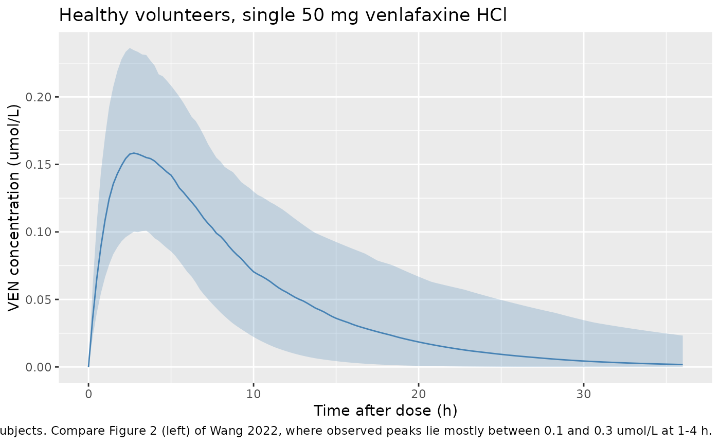
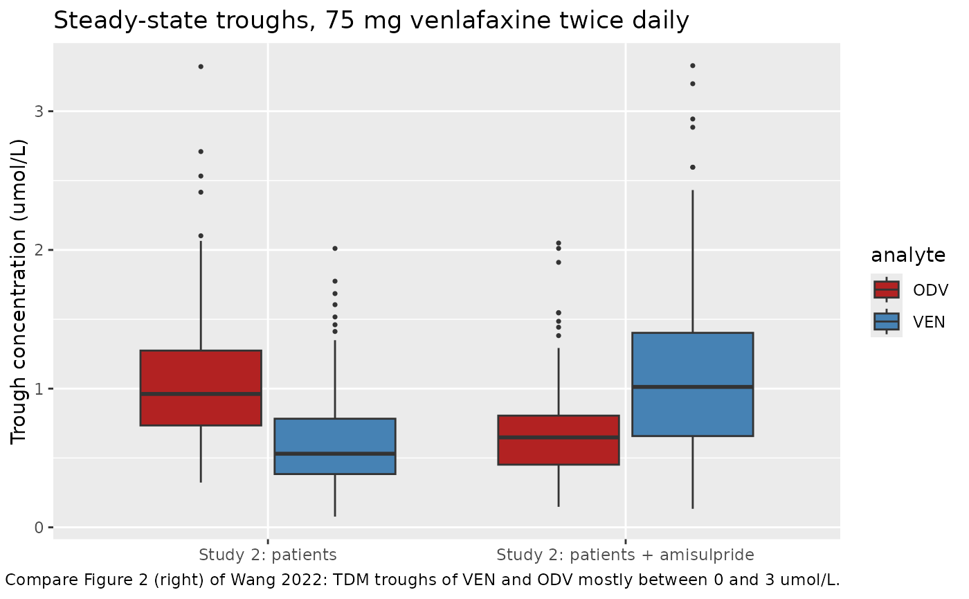
Figure 2 (right): Study 2 troughs
troughs <- sim |>
  dplyr::filter(grepl("Study 2", arm), time == t_last + tau) |>
  dplyr::select(id, arm, VEN = Cc, ODV = Cc_odv) |>
  tidyr::pivot_longer(c(VEN, ODV), names_to = "analyte", values_to = "conc")

ggplot(troughs, aes(arm, conc, fill = analyte)) +
  geom_boxplot(outlier.size = 0.6) +
  scale_fill_manual(values = c(VEN = "steelblue", ODV = "firebrick")) +
  labs(
    x = NULL, y = "Trough concentration (umol/L)",
    title = "Steady-state troughs, 75 mg venlafaxine twice daily",
    caption = "Compare Figure 2 (right) of Wang 2022: TDM troughs of VEN and ODV mostly between 0 and 3 umol/L."
  )
troughs |>
  dplyr::group_by(arm, analyte) |>
  dplyr::summarise(
    median = median(conc), p05 = quantile(conc, 0.05), p95 = quantile(conc, 0.95),
    .groups = "drop"
  ) |>
  dplyr::rename(
    "Arm" = arm, "Analyte" = analyte, "Median (umol/L)" = median,
    "5th percentile" = p05, "95th percentile" = p95
  ) |>
knitr::kable(digits = 2, caption = "Simulated steady-state troughs.")| Arm | Analyte | Median (umol/L) | 5th percentile | 95th percentile |
|---|---|---|---|---|
| Study 2: patients | ODV | 0.96 | 0.46 | 1.97 |
| Study 2: patients | VEN | 0.53 | 0.20 | 1.24 |
| Study 2: patients + amisulpride | ODV | 0.65 | 0.29 | 1.26 |
| Study 2: patients + amisulpride | VEN | 1.01 | 0.39 | 2.33 |
Figure 3: individual clearances by group
indiv <- sim |>
  dplyr::distinct(id, arm, cl, cl_odv) |>
  dplyr::mutate(arm = factor(arm, levels = unique(arm)))

indiv |>
  tidyr::pivot_longer(c(cl, cl_odv), names_to = "parameter", values_to = "value") |>
  dplyr::filter(!(grepl("Study 1", arm) & parameter == "cl_odv")) |>
  dplyr::mutate(parameter = dplyr::recode(
    parameter,
    cl = "VEN CL/F (L/h)", cl_odv = "ODV CL/F (L/h)"
  )) |>
  ggplot(aes(arm, value)) +
  geom_boxplot(fill = "grey80") +
  facet_wrap(~parameter, scales = "free_y") +
  labs(
    x = NULL, y = "Individual clearance (L/h)",
    caption = "Replicates Figure 3 of Wang 2022 (individual estimates by health status and amisulpride use)."
  ) +
  theme(axis.text.x = element_text(angle = 20, hjust = 1))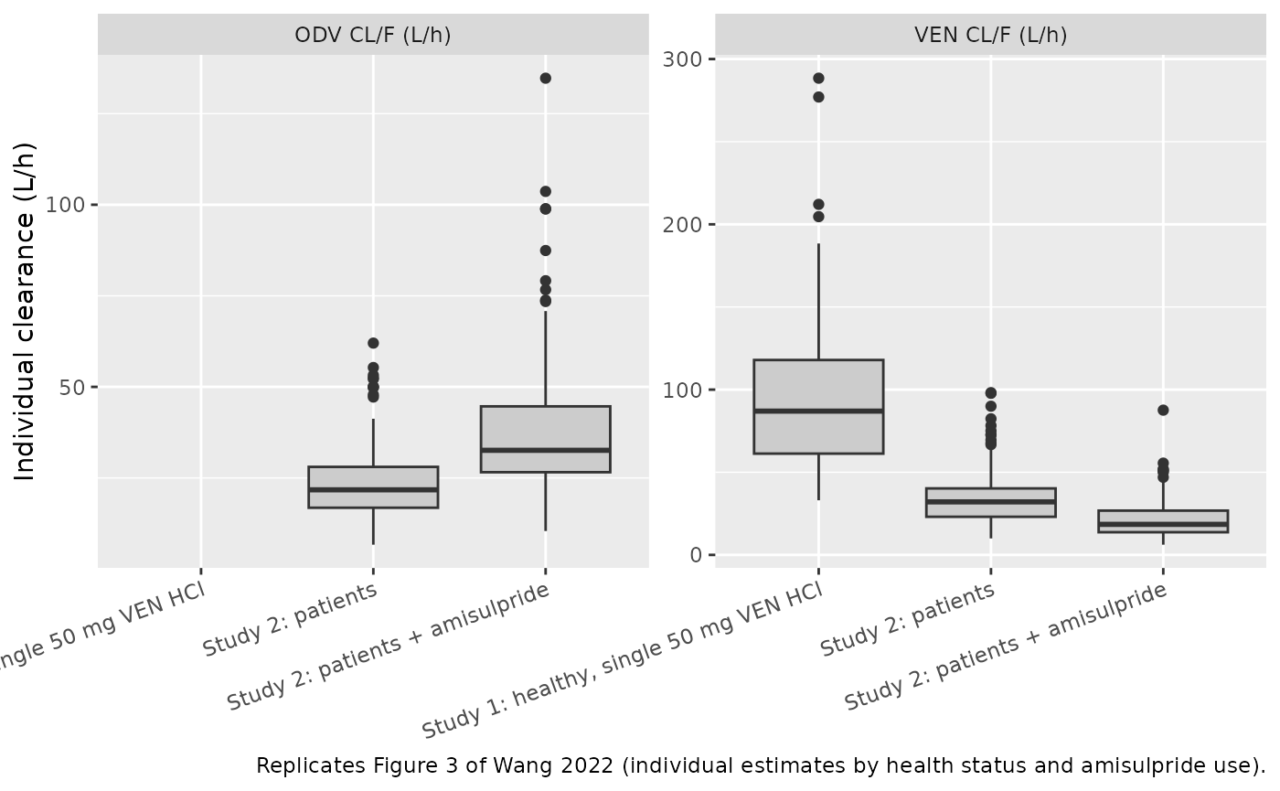
fig3 <- tibble::tribble(
  ~arm, ~parameter, ~fig3_median,
  "Study 1: healthy, single 50 mg VEN HCl", "cl", 80,
  "Study 2: patients", "cl", 32,
  "Study 2: patients + amisulpride", "cl", 19,
  "Study 2: patients", "cl_odv", 22.5,
  "Study 2: patients + amisulpride", "cl_odv", 38.5
)

# Typical values from the packaged parameters: no simulation noise, so the
# comparison tests only the covariate form against the figure.
th <- rxode2::rxode(mod)$theta
#> ℹ parameter labels from comments will be replaced by 'label()'
tv <- tibble::tribble(
  ~arm, ~parameter, ~typical,
  "Study 1: healthy, single 50 mg VEN HCl", "cl", exp(th[["lcl"]]),
  "Study 2: patients", "cl", exp(th[["lcl"]]) * (1 - th[["e_patient_cl"]]),
  "Study 2: patients + amisulpride", "cl",
  exp(th[["lcl"]]) * (1 - th[["e_patient_cl"]]) * (1 - th[["e_conmed_amisulpride_cl"]]),
  "Study 2: patients", "cl_odv", exp(th[["lcl_odv"]]),
  "Study 2: patients + amisulpride", "cl_odv",
  exp(th[["lcl_odv"]]) * (1 + th[["e_conmed_amisulpride_cl_odv"]])
)

cl_cmp <- indiv |>
  tidyr::pivot_longer(c(cl, cl_odv), names_to = "parameter", values_to = "value") |>
  dplyr::group_by(arm, parameter) |>
  dplyr::summarise(sim_median = median(value), .groups = "drop") |>
  dplyr::mutate(arm = as.character(arm)) |>
  dplyr::inner_join(tv, by = c("arm", "parameter")) |>
  dplyr::inner_join(fig3, by = c("arm", "parameter")) |>
  dplyr::mutate(pct_diff = 100 * (typical / fig3_median - 1))

cl_cmp |>
  dplyr::rename(
    "Group" = arm, "Parameter" = parameter,
    "Simulated median (L/h)" = sim_median,
    "Typical value (L/h)" = typical,
    "Figure 3 median, digitised (L/h)" = fig3_median,
    "Typical vs Figure 3 (%)" = pct_diff
  ) |>
knitr::kable(digits = 1, caption = "Individual clearance by group: model vs Figure 3.")| Group | Parameter | Simulated median (L/h) | Typical value (L/h) | Figure 3 median, digitised (L/h) | Typical vs Figure 3 (%) |
|---|---|---|---|---|---|
| Study 1: healthy, single 50 mg VEN HCl | cl | 87.0 | 80.9 | 80.0 | 1.1 |
| Study 2: patients | cl | 32.1 | 31.0 | 32.0 | -3.2 |
| Study 2: patients | cl_odv | 21.7 | 22.1 | 22.5 | -1.8 |
| Study 2: patients + amisulpride | cl | 18.5 | 18.8 | 19.0 | -0.8 |
| Study 2: patients + amisulpride | cl_odv | 32.6 | 35.2 | 38.5 | -8.6 |
stopifnot(
  # A wrong covariate form or sign moves a group value by 40-60 percent.
  # The figure medians carry a few percent of reading error, and the
  # amisulpride group of Figure 3 has only about seven patients, which is
  # why its ODV clearance (typical 35.2 vs about 38.5 L/h) sits furthest off.
  all(abs(cl_cmp$pct_diff) < 15),
  # The simulated cohort medians agree with the typical values.
  abs(median(log(cl_cmp$sim_median / cl_cmp$typical))) < 0.1
)
The amisulpride arm combines the patient and amisulpride effects multiplicatively (80.9 x 0.383 x 0.608 = 18.8 L/h), which lands on the Figure 3 median of about 19 L/h. ODV clearance with amisulpride is the least well matched group (typical 35.2 L/h against a Figure 3 median of about 38.5 L/h), which is unsurprising for a box built from about seven patients’ sparse troughs.
PKNCA validation
Study 1: VEN after a single dose
nca_conc1 <- sim |>
  dplyr::filter(grepl("Study 1", arm), !is.na(Cc)) |>
  dplyr::select(id, time, Cc, arm)
nca_conc1 <- dplyr::bind_rows(
  nca_conc1,
  nca_conc1 |> dplyr::distinct(id, arm) |> dplyr::mutate(time = 0, Cc = 0)
) |>
  dplyr::distinct(id, arm, time, .keep_all = TRUE) |>
  dplyr::arrange(id, time)

dose1 <- events |>
  dplyr::filter(evid == 1, grepl("Study 1", arm)) |>
  dplyr::select(id, time, amt, arm)

nca1 <- PKNCA::pk.nca(PKNCA::PKNCAdata(
  PKNCA::PKNCAconc(nca_conc1, Cc ~ time | arm + id),
  PKNCA::PKNCAdose(dose1, amt ~ time | arm + id),
  intervals = data.frame(
    start = 0, end = Inf,
    cmax = TRUE, tmax = TRUE, aucinf.obs = TRUE, half.life = TRUE
  )
))

published <- tibble::tribble(
  ~arm, ~half.life,
  "Study 1: healthy, single 50 mg VEN HCl", 5.4
)

cmp <- nlmixr2lib::ncaComparisonTable(
  simulated = nca1,
  reference = published,
  by = "arm",
  units = c(cmax = "umol/L", tmax = "h", aucinf.obs = "umol*h/L", half.life = "h"),
  tolerance_pct = 20
)
knitr::kable(
  cmp,
  caption = "Simulated vs published VEN half-life in healthy volunteers (Wang 2022 Discussion: 5.4 h). * differs by more than 20%."
)| NCA parameter | arm | Reference | Simulated | % diff |
|---|---|---|---|---|
| t½ (h) | Study 1: healthy, single 50 mg VEN HCl | 5.4 | 5.08 | -6.0% |
res1 <- as.data.frame(nca1$result)
cmax1 <- res1$PPORRES[res1$PPTESTCD == "cmax"]
hl1 <- res1$PPORRES[res1$PPTESTCD == "half.life"]
stopifnot(
  # Figure 2 (left): observed peaks lie mostly within 0.1-0.3 umol/L. A dose
  # entered in mg instead of umol, or a missed salt correction, moves this
  # far outside the band.
  median(cmax1) > 0.1, median(cmax1) < 0.3,
  # Typical half-life log(2) * V / CL = 5.38 h against the 5.4 h quoted.
  abs(median(hl1) / 5.4 - 1) < 0.15
)
Study 2: steady-state mass balance
All venlafaxine ends up as ODV in this model (first-pass fraction FP
plus all systemic VEN clearance), so at steady state the ODV exposure
over one dosing interval satisfies
dose / AUCtau(ODV) = CL_odv/F for every subject, and the
VEN exposure satisfies
(1 - FP) * dose / AUCtau(VEN) = CL/F. PKNCA recovers both
from the simulated profiles.
ss <- sim |>
  dplyr::filter(grepl("Study 2", arm), time >= t_last) |>
  dplyr::mutate(time = time - t_last)
dose2 <- ss |>
  dplyr::distinct(id, arm) |>
  dplyr::mutate(time = 0, amt = dose_study2)

nca_ss <- function(conc_col) {
  conc <- ss |>
    dplyr::filter(!is.na(.data[[conc_col]])) |>
    dplyr::select(id, time, arm, conc = dplyr::all_of(conc_col))
  res <- PKNCA::pk.nca(PKNCA::PKNCAdata(
    PKNCA::PKNCAconc(conc, conc ~ time | arm + id),
    PKNCA::PKNCAdose(dose2, amt ~ time | arm + id),
    intervals = data.frame(start = 0, end = tau, auclast = TRUE, cmax = TRUE, cmin = TRUE)
  ))
  as.data.frame(res$result) |>
    dplyr::filter(PPTESTCD == "auclast") |>
    dplyr::select(id, arm, auc = PPORRES)
}

indiv_ss <- indiv |>
  dplyr::mutate(arm = as.character(arm)) |>
  dplyr::filter(grepl("Study 2", arm))
mb <- dplyr::inner_join(
  nca_ss("Cc") |> dplyr::rename(auc_ven = auc),
  nca_ss("Cc_odv") |> dplyr::rename(auc_odv = auc),
  by = c("id", "arm")
) |>
  dplyr::inner_join(indiv_ss, by = c("id", "arm")) |>
  dplyr::mutate(
    cl_ven_nca = (1 - 0.048) * dose_study2 / auc_ven,
    cl_odv_nca = dose_study2 / auc_odv,
    pct_ven = 100 * (cl_ven_nca / cl - 1),
    pct_odv = 100 * (cl_odv_nca / cl_odv - 1)
  )

mb |>
  dplyr::group_by(arm) |>
  dplyr::summarise(
    median_cl_ven = median(cl_ven_nca), median_cl_odv = median(cl_odv_nca),
    p90_abs_pct_ven = quantile(abs(pct_ven), 0.9), p90_abs_pct_odv = quantile(abs(pct_odv), 0.9),
    .groups = "drop"
  ) |>
  dplyr::rename(
    "Arm" = arm,
    "Median VEN CL/F from NCA (L/h)" = median_cl_ven,
    "Median ODV CL/F from NCA (L/h)" = median_cl_odv,
    "VEN: 90th percentile of absolute difference (%)" = p90_abs_pct_ven,
    "ODV: 90th percentile of absolute difference (%)" = p90_abs_pct_odv
  ) |>
knitr::kable(digits = 2, caption = "Steady-state mass balance per subject.")| Arm | Median VEN CL/F from NCA (L/h) | Median ODV CL/F from NCA (L/h) | VEN: 90th percentile of absolute difference (%) | ODV: 90th percentile of absolute difference (%) |
|---|---|---|---|---|
| Study 2: patients | 32.1 | 21.75 | 0.03 | 0.01 |
| Study 2: patients + amisulpride | 18.5 | 32.60 | 0.03 | 0.05 |
stopifnot(
  # Both sides use the same drawn parameters; the difference is trapezoidal
  # error on a 0.25 h grid plus a residual approach to steady state for the
  # few subjects with half-lives of several days.
  quantile(abs(mb$pct_ven), 0.9) < 1,
  quantile(abs(mb$pct_odv), 0.9) < 1,
  # Patients without amisulpride: median VEN CL/F 31 L/h and ODV CL/F 22 L/h
  # (Results 3.2 and Table 2).
  abs(median(mb$cl_ven_nca[mb$arm == "Study 2: patients"]) / 31 - 1) < 0.1,
  abs(median(mb$cl_odv_nca[mb$arm == "Study 2: patients"]) / 22.1 - 1) < 0.1
)
Assumptions and deviations
- IIV scale. Table 2 labels the random-effect column “%CV” but prints fractions. The maintainers read these as OMEGA variances because the spread of the individual clearances in Figure 3 matches only that reading (see “Variance scale of the IIV column” above). The large ODV volume variance (1.38, log-SD 1.17) is carried as printed.
- Residual error scale. The residual rows (0.123 VEN, 0.101 ODV) share the mislabelled column and are read on the same scale, as SIGMA variances, giving proportional SDs of 0.351 and 0.318. No figure in the paper tests this directly; 12 percent and 10 percent proportional SDs (the SD reading) would be unusually small for a TDM data set with uncertain dosing times.
- Error model. Results 3.2 mentions a “mixture error” model, but Methods 2.2 and Table 2 give a proportional error for each analyte only; the proportional form is used.
- Covariate combination. The paper does not print the covariate equations. The patient and amisulpride effects are applied as linear fractional changes combined multiplicatively. This reproduces the 31 L/h patient clearance quoted in Results 3.2 and the Figure 3 medians.
- Molar dosing and salt. The figures are in umol/L, so the model is in umol. The Study 1 dose of 50 mg venlafaxine hydrochloride is 159.3 umol. For the Study 2 simulation, the 75 mg doses are taken as venlafaxine base (270.4 umol); the paper does not say whether Study 2 doses were recorded as salt or base.
- Formulation. Study 2 patients mostly took sustained-release tablets, but formulation was not a significant covariate and the model has one absorption rate (0.63 1/h, fixed from an unpublished two-compartment VEN model). The simulated Study 2 profiles therefore have immediate-release absorption.
- Fraction converted pre-systemically. FP is estimated directly (0.048) as a fraction of the absorbed dose, with no IIV.
- No erratum or correction notice for the article was found on Europe PMC (checked 2026-10-10).