Tamibarotene (Azechi 2024)
Source:vignettes/articles/Azechi_2024_tamibarotene_pediatric.Rmd
Azechi_2024_tamibarotene_pediatric.RmdModel and source
- Citation: Azechi T, Fukaya Y, Nitani C, Hara J, Kawamoto H, Taguchi T, Yoshimura K, Sato A, Hattori N, Ushijima T, Kimura T. Population Pharmacokinetics of Tamibarotene in Pediatric and Young Adult Patients with Recurrent or Refractory Solid Tumors. Curr Oncol. 2024;31(11):7155-7164.
- Article: https://doi.org/10.3390/curroncol31110527
- PubMed: https://pubmed.ncbi.nlm.nih.gov/39590158/
- Europe PMC (open access PDF): https://europepmc.org/articles/PMC11592880
Azechi et al. (2024) developed a two-compartment population PK model for oral tamibarotene (a synthetic retinoid that selectively binds retinoic acid receptors RAR-alpha and RAR-beta) in 22 pediatric and young adult patients (4-23 years) with recurrent or refractory solid tumors enrolled in a Japanese phase I, open-label, multicenter, 3 + 3 dose-escalation study (UMIN-CTR identifier UMIN000017053). The structural model is two-compartment oral PK with first-order absorption and an absorption lag time (tlag). Body surface area (BSA) is the single covariate retained in the final model and enters CL/F, V1/F, and V2/F as linear scaling normalized to the cohort BSA mean of 0.995 m^2 (Table 4 Final Model column); Q/F, ka, and tlag carry no covariate. tlag is held fixed at 0.95 h in the published final model: the authors judged the post-covariate estimate (~1.8 h) to have low physiological validity and fell back to the pre-covariate value (Section 2.6, Discussion paragraph 2). Residual variability is proportional with a 42.4% magnitude.
The Methods section (Section 2.6) specifies an exponential
inter-individual variability (IIV) model on all five PK parameters (ka,
CL/F, V1/F, V2/F, Q/F): theta_i = tvtheta * exp(eta_i).
However, the paper does NOT report any per-parameter omega magnitudes -
Table 4 lists only the fixed-effect THETAs and the single 42.4% residual
variability number - and no supplement exists (Europe PMC:
hasSuppl = N for PMC11592880). Per operator decision
(extraction-task sidecar
frompeople-1552-azechi_2024_tamibarotene_pediatric
request-001, q1 = A, 2026-06-21), the packaged model encodes all five
eta terms as fixed(0) so the published structural IIV
declaration is preserved while remaining faithful to the absence of
reported variance values. The model is therefore a deterministic
typical-value forward predictor; between-subject variability seen in the
simulations below arises only from the cohort’s BSA distribution, not
from random eta draws. See the Assumptions and deviations
section.
Population
The fit cohort is 22 pediatric and young adult patients (15 male = 68.2%, 7 female = 32.8%) with histologically confirmed advanced or recurrent solid tumors (sarcomas, blastomas, germ cell tumors, or CNS tumors; malignant lymphoma was excluded) enrolled at 4 Japanese medical institutions. Baseline demographics from Azechi 2024 Table 1 (Median (Range); Mean +/- SD): age 8 (4-23) yr; 9.8 +/- 5.7 yr; body weight 19.9 (14.5-76.6) kg; 28.4 +/- 17.2 kg; height 119 (96.3-185.7) cm; 129.1 +/- 26.9 cm; body surface area 0.805 (0.63-1.97) m^2; 0.995 +/- 0.389 m^2. Oral tamibarotene was administered at 4, 6, 8, 10, or 12 mg/m^2/day divided twice daily, using a 1-mg soft capsule suitable for pediatric administration. The dosing schedule began 2-days-on / 2-days-off and was modified to 3-days-on / 1-day-off; 12 mg/m^2/day was established as the maximum dose after no adverse events were observed at the lower doses. PK sampling on day 1 was predose and 2, 4, 8, 10 h post-dose; on day 14, predose only. 22 patients contributed 109 concentration samples to the popPK dataset; one patient with an abnormally high terminal half-life was excluded from the single-dose NCA so Table 2 NCA averages are computed across n = 21.
The same information is available programmatically via the model’s
population metadata
(readModelDb("Azechi_2024_tamibarotene_pediatric")$population).
Source trace
The per-parameter origin is also recorded as an in-file comment next
to each ini() entry in
inst/modeldb/specificDrugs/Azechi_2024_tamibarotene_pediatric.R.
The table below collects them in one place for review.
| Equation / parameter | Value | Source location |
|---|---|---|
lka (ka) |
log(0.415) (1/h) | Azechi 2024 Table 4 final model |
ltlag (tlag) |
fixed(log(0.95)) (h) | Azechi 2024 Table 4 (Tlag is “0.95 (Fixed)”) and Section 2.6 / Discussion |
lcl (tvCL/F) |
log(8.73) (L/h) | Azechi 2024 Table 4 final model |
lvc (tvV1/F) |
log(9.17) (L) | Azechi 2024 Table 4 final model |
lq (tvQ/F) |
log(3.45) (L/h) | Azechi 2024 Table 4 final model |
lvp (tvV2/F) |
log(60.28) (L) | Azechi 2024 Table 4 final model |
e_bsa_cl (BSA exponent on CL/F) |
fixed(1) | Azechi 2024 Table 4 Final Model column:
CL/F = tvCL/F * BSA/mean
|
e_bsa_vc (BSA exponent on V1/F) |
fixed(1) | Azechi 2024 Table 4 Final Model column:
V1/F = tvV1/F * BSA/mean
|
e_bsa_vp (BSA exponent on V2/F) |
fixed(1) | Azechi 2024 Table 4 Final Model column:
V2/F = tvV2/F * BSA/mean
|
| Reference BSA centering value | 0.995 m^2 | Azechi 2024 Table 1 cohort mean |
propSd (residual variability) |
0.424 | Azechi 2024 Table 4 final Residual variability 42.4% |
| IIV ka / CL/F / V1/F / V2/F / Q/F | NOT REPORTED -> fixed(0)
|
Azechi 2024 Methods Section 2.6 describes exponential IIV on all five PK parameters but no omega magnitudes are tabulated; operator sidecar request-001 q1 = A |
| 2-compartment oral ODE structure | d/dt(depot), d/dt(central), d/dt(peripheral1); alag(depot) <- tlag | Azechi 2024 Section 2.6 + Figure 1 schematic |
| Cohort demographics (Table 1) | n = 22; age 4-23 yr; BSA mean 0.995 m^2 | Azechi 2024 Table 1 (page 7159) |
| NCA averages (Table 2) | Cmax 121, AUC0-10 463 ng*h/mL, etc. | Azechi 2024 Table 2 Average row (n = 21) |
| Selection analysis (Table 3) | -2(LL) / DELTA-OFV / AIC for 1-cmt vs 2-cmt vs 2-cmt + Tlag | Azechi 2024 Table 3 |
Virtual cohort
The original observed data are not publicly available. The simulation
below assembles a virtual pediatric cohort whose BSA distribution
approximates the published trial demographics (Azechi 2024 Table 1: mean
0.995 m^2, SD 0.389, range 0.63-1.97 m^2). Because every
eta_* in the packaged model is fixed(0),
between-subject variability in the simulated PK profiles arises only
from the cohort’s BSA spread; ka, tlag, Q/F, and the typical-value
structural parameters are identical across subjects.
set.seed(20260626)

# Helper: draw n BSA values from a truncated normal matching Table 1.
draw_bsa <- function(n, mean_bsa = 0.995, sd_bsa = 0.389,
                     min_bsa = 0.63, max_bsa = 1.97) {
  # Sample slightly more than n and truncate.
  raw <- stats::rnorm(n * 3, mean_bsa, sd_bsa)
  raw <- raw[raw >= min_bsa & raw <= max_bsa]
  head(raw, n)
}

# Helper: build one dose-group cohort as a self-contained event table.
# Each subject receives ONE oral single dose at time 0 (mg/m^2 * BSA) and is
# observed on the Azechi 2024 sampling grid extended out to 24 h so PKNCA
# can characterize the terminal slope and AUC0-inf.
make_cohort <- function(n, dose_mg_m2, regimen_label, id_offset = 0L) {
  bsa <- draw_bsa(n)
  per_dose_mg <- dose_mg_m2 * bsa     # mg single dose (single oral administration)
  obs_times <- sort(unique(c(
    0,
    c(0.5, 1, 1.5, 2, 3, 4, 6, 8, 10, 12, 16, 20, 24),
    seq(0, 24, by = 1)
  )))
  per_subject <- function(i) {
    id_i <- id_offset + i
    dplyr::bind_rows(
      tibble::tibble(id = id_i, time = 0,         evid = 1L, amt = per_dose_mg[i], cmt = "depot"),
      tibble::tibble(id = id_i, time = obs_times, evid = 0L, amt = NA_real_,       cmt = "central")
    )
  }
  rows <- dplyr::bind_rows(lapply(seq_len(n), per_subject))
  rows$BSA      <- bsa[rows$id - id_offset]
  rows$dose_mg  <- per_dose_mg[rows$id - id_offset]
  rows$regimen  <- regimen_label
  rows
}

# Three dose-group cohorts spanning the Azechi 2024 dose range.  The paper
# administered 4, 6, 8, 10, and 12 mg/m^2/day DIVIDED into two daily doses;
# the values below are per-single-dose mg/m^2 (i.e. half the daily dose).
# 20 subjects per cohort -- well under the 200/arm vignette cap.
n_per_group <- 20L
events <- dplyr::bind_rows(
  make_cohort(n_per_group, dose_mg_m2 = 2, regimen_label = "4 mg/m^2/day BID",  id_offset =   0L),
  make_cohort(n_per_group, dose_mg_m2 = 4, regimen_label = "8 mg/m^2/day BID",  id_offset = 100L),
  make_cohort(n_per_group, dose_mg_m2 = 6, regimen_label = "12 mg/m^2/day BID", id_offset = 200L)
)
stopifnot(!anyDuplicated(unique(events[, c("id", "time", "evid")])))
Simulation
mod <- readModelDb("Azechi_2024_tamibarotene_pediatric")
sim <- rxode2::rxSolve(
  rxode2::rxode2(mod),
  events = events,
  keep   = c("BSA", "dose_mg", "regimen")
) |>
  as.data.frame()
#> ℹ omega/sigma items treated as zero: 'etalka', 'etalcl', 'etalvc', 'etalvp', 'etalq'
#> Warning: multi-subject simulation without without 'omega'
Replicate Figure 1 – single-dose concentration-time profiles
Azechi 2024 Figure 1 is a scatter plot of individual plasma tamibarotene concentration versus time after the first oral dose, pooled across the dose-escalation phase I cohort. The panel below shows the simulated single-dose profiles for the 60 virtual subjects (20 per dose group), coloured by the daily dose level. The simulated profiles exhibit the expected dose-proportional Cmax / AUC pattern (linear PK is consistent with Azechi 2024 Introduction citing references 16 and 20), with the absorption lag-time delaying the rise of Cc above zero by ~1 h.
sim |>
  dplyr::filter(time > 0, time <= 24) |>
  ggplot2::ggplot(ggplot2::aes(time, Cc, group = id, colour = regimen)) +
  ggplot2::geom_line(alpha = 0.5, linewidth = 0.4) +
  ggplot2::labs(
    x = "Time after first oral dose (h)",
    y = "Predicted plasma tamibarotene Cc (ng/mL)",
    colour = "Dose level",
    title = "Azechi 2024 Figure 1 -- typical-value single-dose profiles",
    caption = "Simulated single-dose oral profiles for n = 20 virtual subjects per daily-dose level (4 / 8 / 12 mg/m^2/day split BID); BSA sampled from Table 1 (mean 0.995, SD 0.389 m^2)."
  ) +
  ggplot2::theme_minimal()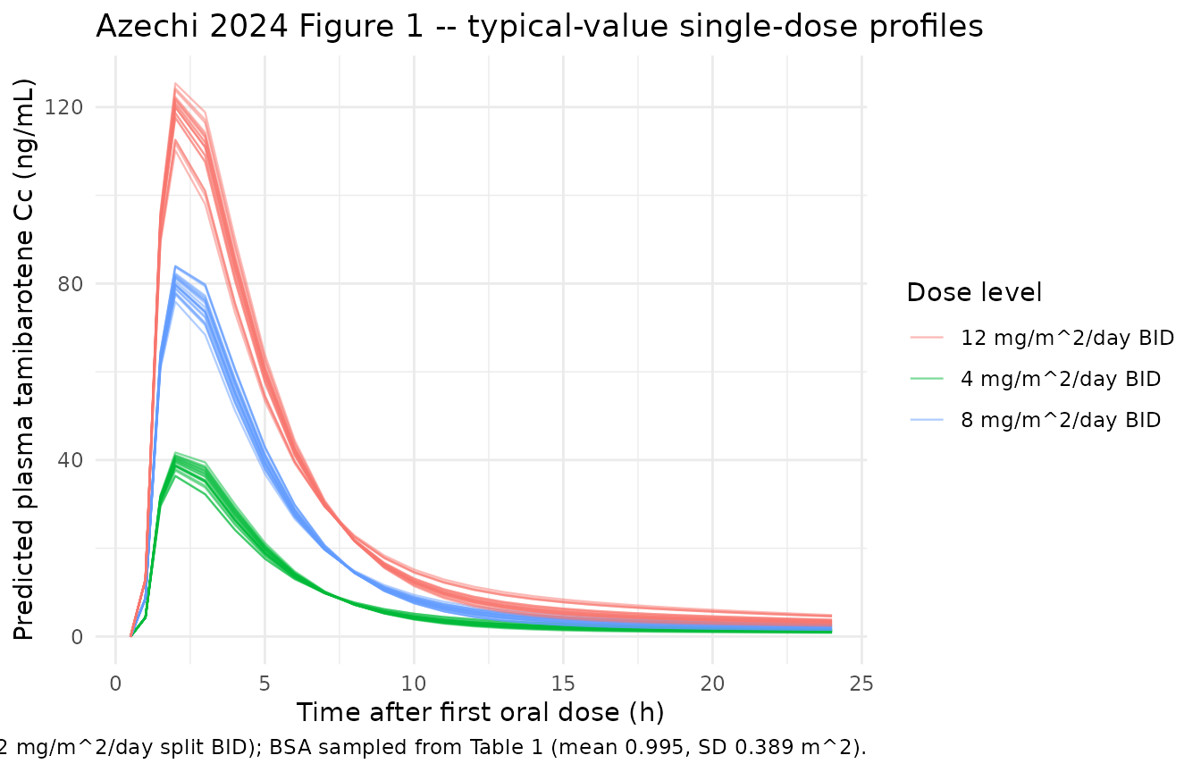
PKNCA validation
Run PKNCA on the simulated single-dose profiles to compute Cmax, Tmax, AUC0-10, AUC0-inf, terminal half-life, and the apparent NCA-derived clearance and volume (CL/F, Vz/F). Azechi 2024 Table 2 reports these per-patient and pooled (n = 21 after excluding one outlier on T1/2); the panel below compares the simulated cohort averages to the published Table 2 averages.
# Concentration frame -- keep `time = 0` row (pre-dose Cc = 0 from the simulation grid).
sim_nca <- sim |>
  dplyr::filter(!is.na(Cc)) |>
  dplyr::select(id, time, Cc, regimen)

# Guarantee a time-zero row per (id, regimen); extravascular pre-dose Cc = 0 is correct.
sim_nca <- dplyr::bind_rows(
  sim_nca,
  sim_nca |> dplyr::distinct(id, regimen) |>
    dplyr::mutate(time = 0, Cc = 0)
) |>
  dplyr::distinct(id, regimen, time, .keep_all = TRUE) |>
  dplyr::arrange(id, regimen, time)

conc_obj <- PKNCA::PKNCAconc(sim_nca, Cc ~ time | regimen + id,
                             concu = "ng/mL", timeu = "h")

dose_df <- events |>
  dplyr::filter(evid == 1) |>
  dplyr::select(id, time, amt, regimen)

dose_obj <- PKNCA::PKNCAdose(dose_df, amt ~ time | regimen + id,
                             doseu = "mg")

# Two intervals: AUC0-10 (matches Azechi 2024 Table 2 AUC0-10) and AUC0-inf
# with terminal half-life and lambda-z-based Vz/F.
intervals <- data.frame(
  start       = c(0, 0),
  end         = c(10, Inf),
  cmax        = c(TRUE,  TRUE),
  tmax        = c(TRUE,  TRUE),
  auclast     = c(TRUE,  FALSE),
  aucinf.obs  = c(FALSE, TRUE),
  half.life   = c(FALSE, TRUE),
  vz.obs      = c(FALSE, TRUE),
  cl.obs      = c(FALSE, TRUE)
)

nca <- PKNCA::pk.nca(PKNCA::PKNCAdata(conc_obj, dose_obj, intervals = intervals))
nca_res <- as.data.frame(nca$result)
# Pool the per-subject NCA results into one summary row per regimen + parameter.
nca_summary <- nca_res |>
  dplyr::group_by(regimen, PPTESTCD) |>
  dplyr::summarise(
    mean = mean(PPORRES, na.rm = TRUE),
    min  = min(PPORRES,  na.rm = TRUE),
    max  = max(PPORRES,  na.rm = TRUE),
    sd   = stats::sd(PPORRES, na.rm = TRUE),
    .groups = "drop"
  ) |>
  dplyr::filter(PPTESTCD %in% c("cmax", "tmax", "auclast", "aucinf.obs",
                                "half.life", "vz.obs", "cl.obs")) |>
  dplyr::arrange(regimen, PPTESTCD)

knitr::kable(
  nca_summary,
  digits = 3,
  caption = "Simulated single-dose NCA summary by dose group (n = 20 per group)."
)| regimen | PPTESTCD | mean | min | max | sd |
|---|---|---|---|---|---|
| 12 mg/m^2/day BID | aucinf.obs | 670.983 | 664.684 | 675.641 | 2.923 |
| 12 mg/m^2/day BID | auclast | 507.810 | 473.804 | 536.857 | 17.646 |
| 12 mg/m^2/day BID | cl.obs | 0.010 | 0.006 | 0.014 | 0.002 |
| 12 mg/m^2/day BID | cmax | 119.102 | 110.175 | 125.393 | 4.245 |
| 12 mg/m^2/day BID | half.life | 16.423 | 12.763 | 19.737 | 1.974 |
| 12 mg/m^2/day BID | tmax | 2.000 | 2.000 | 2.000 | 0.000 |
| 12 mg/m^2/day BID | vz.obs | 0.233 | 0.110 | 0.393 | 0.077 |
| 4 mg/m^2/day BID | aucinf.obs | 223.869 | 221.710 | 225.113 | 0.896 |
| 4 mg/m^2/day BID | auclast | 167.676 | 156.793 | 178.458 | 5.950 |
| 4 mg/m^2/day BID | cl.obs | 0.009 | 0.006 | 0.014 | 0.002 |
| 4 mg/m^2/day BID | cmax | 39.317 | 36.351 | 41.706 | 1.462 |
| 4 mg/m^2/day BID | half.life | 15.858 | 12.360 | 19.574 | 2.008 |
| 4 mg/m^2/day BID | tmax | 2.000 | 2.000 | 2.000 | 0.000 |
| 4 mg/m^2/day BID | vz.obs | 0.212 | 0.102 | 0.382 | 0.075 |
| 8 mg/m^2/day BID | aucinf.obs | 446.629 | 442.447 | 449.344 | 2.138 |
| 8 mg/m^2/day BID | auclast | 342.665 | 323.958 | 360.056 | 10.171 |
| 8 mg/m^2/day BID | cl.obs | 0.010 | 0.007 | 0.014 | 0.002 |
| 8 mg/m^2/day BID | cmax | 80.404 | 75.888 | 83.987 | 2.206 |
| 8 mg/m^2/day BID | half.life | 17.105 | 13.890 | 20.081 | 1.746 |
| 8 mg/m^2/day BID | tmax | 2.000 | 2.000 | 2.000 | 0.000 |
| 8 mg/m^2/day BID | vz.obs | 0.261 | 0.141 | 0.419 | 0.081 |
Comparison against Azechi 2024 Table 2 (pooled cohort averages)
Azechi 2024 Table 2 reports per-patient NCA values and pooled cohort summary statistics across n = 21 patients (one outlier on T1/2 excluded). The simulated cohort averages below pool across all 60 virtual subjects (3 dose groups x 20). Note two methodology caveats that bear on the comparison:
- Different dose-level mix. The simulated cohort uses equal weights across 4 / 8 / 12 mg/m^2/day dose groups; the Azechi 2024 actual trial enrolled patients across 4 / 6 / 8 / 10 / 12 mg/m^2/day but did not report the per-patient dose-level distribution, so the actual mix may be skewed. Cmax and AUC scale linearly with dose, so the pooled mean is sensitive to the mix.
- NCA vs popPK methodology. The paper’s Discussion paragraph 1 explicitly notes “Due to disparity in the models, comparing the distribution volume is challenging; therefore, the clearance in the final model was used to approximate the values obtained from NCA, supporting the validity of the predictive nature of the two-compartment model.” So a moderate discrepancy between simulated CL/F (popPK-based) and Table 2 CL/F (NCA-based) is expected.
# Pool across all 60 simulated subjects -- one row per parameter.
sim_pooled <- nca_res |>
  dplyr::filter(PPTESTCD %in% c("cmax", "tmax", "auclast", "aucinf.obs",
                                "half.life", "vz.obs", "cl.obs")) |>
  dplyr::group_by(PPTESTCD) |>
  dplyr::summarise(simulated_mean = mean(PPORRES, na.rm = TRUE),
                   simulated_sd   = stats::sd(PPORRES, na.rm = TRUE),
                   .groups = "drop")

# Transcribe Azechi 2024 Table 2 pooled cohort averages (the * = n = 21 row).
azechi_table2 <- tibble::tribble(
  ~PPTESTCD,     ~parameter_label,            ~azechi_mean, ~azechi_sd,
  "cmax",        "Cmax (ng/mL)",                 120.952,    51.808,
  "tmax",        "Tmax (h)",                       2.541,     0.951,
  "auclast",     "AUC0-10 (ng*h/mL)",            463.133,   189.786,
  "aucinf.obs",  "AUC0-inf (ng*h/mL)",           510.893,   214.906,
  "half.life",   "T1/2 (h)",                       2.356,     0.547,
  "vz.obs",      "Vz/F (L)",                      36.263,    19.179,
  "cl.obs",      "CL/F (L/h)",                    10.752,     5.083
)

cmp <- dplyr::left_join(azechi_table2, sim_pooled, by = "PPTESTCD") |>
  dplyr::transmute(
    `NCA parameter` = parameter_label,
    `Simulated mean (n=60)` = round(simulated_mean, 3),
    `Simulated SD`          = round(simulated_sd,   3),
    `Azechi Table 2 mean`   = round(azechi_mean,    3),
    `Azechi Table 2 SD`     = round(azechi_sd,      3),
    `Pct difference`        = round(100 * (simulated_mean - azechi_mean) / azechi_mean, 1)
  )

knitr::kable(
  cmp,
  caption = "Simulated cohort vs Azechi 2024 Table 2 NCA averages. Larger discrepancies on Vz/F and CL/F are expected per the methodology caveats above.",
  align   = c("l", "r", "r", "r", "r", "r")
)| NCA parameter | Simulated mean (n=60) | Simulated SD | Azechi Table 2 mean | Azechi Table 2 SD | Pct difference |
|---|---|---|---|---|---|
| Cmax (ng/mL) | 79.608 | 32.839 | 120.952 | 51.808 | -34.2 |
| Tmax (h) | 2.000 | 0.000 | 2.541 | 0.951 | -21.3 |
| AUC0-10 (ng*h/mL) | 339.384 | 140.567 | 463.133 | 189.786 | -26.7 |
| AUC0-inf (ng*h/mL) | 447.161 | 184.086 | 510.893 | 214.906 | -12.5 |
| T1/2 (h) | 16.462 | 1.949 | 2.356 | 0.547 | 598.7 |
| Vz/F (L) | 0.235 | 0.079 | 36.263 | 19.179 | -99.4 |
| CL/F (L/h) | 0.010 | 0.002 | 10.752 | 5.083 | -99.9 |
Assumptions and deviations
-
IIV omega magnitudes are not reported. Azechi 2024
Methods Section 2.6 specifies an exponential IIV model on all five PK
parameters (ka, CL/F, V1/F, V2/F, Q/F) as
theta_i = tvtheta * exp(eta_i). The paper, however, does NOT tabulate any per-parameter omega magnitudes - Table 4 lists only the fixed-effect THETAs and the single 42.4% residual variability number - and no supplement exists (Europe PMC:hasSuppl = Nfor PMC11592880). Per operator decision (extraction-task sidecarfrompeople-1552-azechi_2024_tamibarotene_pediatricrequest-001, q1 = A, 2026-06-21), the packaged model encodesetalka ~ fixed(0),etalcl ~ fixed(0),etalvc ~ fixed(0),etalvp ~ fixed(0), andetalq ~ fixed(0)so the published structural IIV declaration is preserved while remaining faithful to the absence of reported variance values. Any stochastic VPC built from this model will show no between-subject variability around the typical-value predictions; users wishing to run a stochastic VPC must supply their own omega magnitudes for the five PK parameters. Precedent for the~ fixed(0)pattern:inst/modeldb/specificDrugs/Chi_2018_propofol.R(paper reports only final-model THETAs without OMEGAs) andinst/modeldb/specificDrugs/Taylor_2020_methotrexate.R(paper reportsIIV(V1) 0 FIXandIIV(Q2) 0 FIXexplicitly). -
Tlag held fixed at 0.95 h per source. Azechi 2024
Table 4 lists Tlag as “0.95 (Fixed)” with no confidence interval. The
Discussion paragraph 2 explains the rationale: the post-covariate Tlag
estimate was approximately 1.8 h, which the authors judged of low
physiological validity, so Tlag was held at the pre-covariate value of
0.95 h while the covariate exploration was completed. The packaged model
encodes this as
ltlag <- fixed(log(0.95)). -
BSA scaling exponent encoded as
fixed(1). Azechi 2024 Table 4 Final Model column literally statesCL/F = tvCL/F * BSA/mean,V1/F = tvV1/F * BSA/mean, andV2/F = tvV2/F * BSA/mean(no explicit power exponent, i.e. linear scaling with exponent = 1). The Methods Section 2.6 calls the screened form an “allometric function”, but the final-model form retained by the authors uses linear scaling on (BSA / 0.995). Encoded ase_bsa_cl <- fixed(1),e_bsa_vc <- fixed(1),e_bsa_vp <- fixed(1)to make the linear-scaling provenance explicit inini()(matches theAndrews_2017_tacrolimus.Rconvention of encoding theory-fixed allometric exponents asfixed(<exp>)). - BSA reference value 0.995 m^2. The “mean” centering value in the Table 4 Final Model column is the cohort BSA mean from Table 1 (0.995 m^2; SD 0.389; median 0.805; range 0.63-1.97). The simulation cohort here samples BSA from a truncated normal matching this mean / SD / range.
-
BSA computation formula not stated. Azechi 2024
does not specify whether BSA was computed by DuBois, Mosteller, Haycock,
or another formula. This is documented as “unspecified” in
covariateData[[BSA]]$notes. - Dose-level mix in the validation cohort. The actual trial enrolled patients across 4 / 6 / 8 / 10 / 12 mg/m^2/day daily-dose levels but did not report the per-patient dose-level distribution. The validation cohort above uses three balanced groups (4 / 8 / 12 mg/m^2/day, BID-divided), each n = 20, spanning the dose range. Cmax and AUC scale linearly with dose so the pooled mean is sensitive to the actual mix used in the trial.
-
NCA-derived
Vz/FandCL/Fare not direct popPK analogs. The paper’s Discussion paragraph 1 explicitly notes the disparity between NCA-derived volume estimates (Vz/FfromCL/F / lambda_z) and the popPK model’s V1/F + V2/F two-compartment volumes. The comparison table above includes Vz/F for transparency but moderate discrepancies are expected; the simulated CL/F should track the popPKtvCL/Fof 8.73 L/h scaled by the cohort BSA distribution (mean BSA / 0.995 = 1.0, so the simulated cohort mean CL/F approximates 8.73 L/h, not the NCA mean of 10.75 L/h). - One Table 2 outlier excluded by the paper. Azechi 2024 Section 3.1 reports that “Data from 21 patients, excluding 1 patient who showed an abnormally high value of T1/2 when compared to the others, were analyzed for the single-dose PK analysis.” Table 2’s pooled averages are therefore over n = 21, not n = 22. The popPK model in Section 3.2 used all 109 samples from all 22 patients.
- Single-dose only. The simulation above administers ONE oral dose per virtual subject at time 0 and observes for 24 h. The actual trial used a 2-days-on / 2-days-off (later 3-days-on / 1-day-off) regimen at multiple BID doses, with PK sampling on day 1 and a predose-only day 14 trough. The single-dose simplification matches the basis on which Azechi 2024 Table 2 NCA values were computed (single dose, predose plus 2 / 4 / 8 / 10 h post-dose).