Daptomycin (Garcia-Martinez 2022)
Source:vignettes/articles/GarciaMartinez_2022_daptomycin.Rmd
GarciaMartinez_2022_daptomycin.RmdModel and source
- Citation: Garcia-Martinez T, Belles-Medall MD, Garcia-Cremades M, Ferrando-Piqueres R, Mangas-Sanjuan V, Merino-Sanjuan M. Population pharmacokinetic/pharmacodynamic modelling of daptomycin for schedule optimization in patients with renal impairment. Pharmaceutics. 2022;14(10):2226. doi:10.3390/pharmaceutics14102226.
- Description: Two-compartment population PK model for intravenous daptomycin in hospitalised adults with normal renal function or renal impairment (46 patients, 157 steady-state serum concentrations, 4-12 mg/kg q24h as a 30-min infusion; two Spanish hospitals). The ODE system describes UNBOUND daptomycin with linear elimination and linear peripheral distribution; the observed total serum concentration is reconstructed algebraically from a single-site saturable protein-binding equation Ctotal = Cu + Bmax * Cu / (KD + Cu). Unbound clearance scales with Cockcroft-Gault creatinine clearance by a power function centred on 92.8 mL/min/1.73 m^2. Log-normal IIV on unbound clearance and unbound peripheral volume; residual error is additive on the log scale.
- Article (open access): https://doi.org/10.3390/pharmaceutics14102226
The ODE system describes unbound daptomycin. Total serum daptomycin, the only measured quantity, is reconstructed algebraically from the single-site saturable binding relationship of the paper’s Equation 2,
so the bound drug is not a mass-balance state. The model exposes the
unbound concentration as Cunbound and the total as
Cc (the observation). With Bmax = 160 mg/L and
KD = 3.56 mg/L the unbound fraction is about 2% at
trough-level concentrations and rises steeply as binding saturates near
the end of an infusion; this is why the paper’s efficacy targets are
expressed on unbound AUC.
Population
Garcia-Martinez 2022 studied 46 adults (43 men, 93%) receiving daptomycin for Gram-positive infection in two Spanish hospitals (Table 1). Median (IQR) age was 68 (59-81) years, body weight 75 (65-85) kg, serum albumin 2.9 (2.4-3.4) g/dL and Cockcroft-Gault creatinine clearance 93 (50-136) mL/min/1.73 m^2; 35% had normal renal function, 28% mild, 30% moderate and 7% severe impairment, and patients on renal replacement therapy were excluded. Daptomycin was given as a 30-min infusion every 24 h at 4-12 mg/kg (median 675 mg, 9.1 mg/kg). Five serum samples per patient were drawn from day 4 (steady state): pre-dose, 0.5, 1-2 and 4-10 h after the end of infusion, and before the next dose (157 concentrations in all). Total daptomycin was measured by HPLC-UV; unbound concentrations were not measured.
The same information is available programmatically via
readModelDb("GarciaMartinez_2022_daptomycin")()$population.
Source trace
| Equation / parameter | Value | Source location |
|---|---|---|
| Two-compartment unbound-drug ODEs | n/a | Results 3.2.1 and Figure 1 |
Total = unbound + saturable bound (Cc) |
n/a | Methods, Equation 2; Results 3.2.1 |
cl = CL x (CRCL / 92.8)^0.19 |
n/a | Results 3.2.2, Equation 4 |
lcl (unbound CL) |
log(6.98) L/h | Table 2 |
lvc (unbound V1) |
log(0.95) L | Table 2 |
lq (unbound Q) |
log(1.96) L/h | Table 2 |
lvp (unbound V2) |
log(21) L | Table 2 (unit printed as L/h) |
lbmax |
log(160) mg/L | Table 2; Results 3.2.2 text |
lkd |
log(3.56) mg/L | Table 2; Results 3.2.2 text |
e_crcl_cl |
0.19 | Table 2 ‘CrCl on CL’; Equation 4 |
etalcl |
0.32^2 = 0.1024 | Table 2 IIV ‘CL (%)’ = 32 |
etalvp |
0.47^2 = 0.2209 | Table 2 IIV ‘V2 (%)’ = 47 |
expSd |
0.22 | Table 2 ‘Additive on Log-scale (%)’ = 22 |
Steady-state profile (Figure 2)
The paper’s prediction-corrected VPC (Figure 2) shows total concentrations at steady state after a 30-min infusion: the observed median is about 70 mg/L 1 h after the start of the infusion, about 35 mg/L at 8 h and about 15 mg/L at the 24-h trough. A virtual cohort of 200 patients receiving the cohort median dose of 675 mg q24h for four days, with creatinine clearance drawn log-normally around the Table 1 median and IQR, is compared below.
set.seed(2022)
n_vpc <- 200
crcl_sdlog <- log(136 / 50) / (2 * qnorm(0.75))
vpc_cov <- tibble(
  id = seq_len(n_vpc),
  CRCL = pmin(pmax(exp(rnorm(n_vpc, log(93), crcl_sdlog)), 15), 200)
)
obs_times <- 72 + sort(unique(c(seq(0, 1, by = 0.1), seq(1, 24, by = 0.5))))
vpc_events <- rxode2::et(amt = 675, rate = 675 / 0.5, ii = 24, addl = 3, cmt = "central") |>
  rxode2::et(obs_times, cmt = "central") |>
  as.data.frame() |>
  select(-dplyr::any_of("id")) |>
  tidyr::crossing(vpc_cov) |>
  arrange(id, time, desc(evid))

mod <- readModelDb("GarciaMartinez_2022_daptomycin")
sim_vpc <- rxode2::rxSolve(mod, events = vpc_events, keep = "CRCL") |>
  as.data.frame()
#> ℹ parameter labels from comments will be replaced by 'label()'
sim_vpc |>
  mutate(tad = time - 72) |>
  group_by(tad) |>
  summarise(
    Q025 = quantile(sim, 0.025),
    Q50 = quantile(sim, 0.5),
    Q975 = quantile(sim, 0.975),
    .groups = "drop"
  ) |>
  ggplot(aes(tad, Q50)) +
  geom_ribbon(aes(ymin = Q025, ymax = Q975), fill = "steelblue", alpha = 0.25) +
  geom_line(colour = "steelblue4") +
  scale_y_log10() +
  coord_cartesian(ylim = c(1, 400)) +
  labs(
    x = "Time after last dose (h)",
    y = "Total daptomycin (mg/L)",
    title = "Simulated steady-state profile, 675 mg q24h",
    caption = "Compare with Figure 2 of Garcia-Martinez 2022 (median and 95% interval)."
  )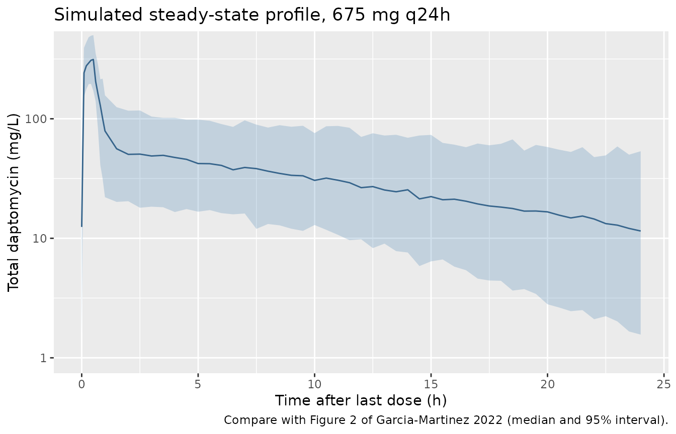
The typical-value profile is the structural check: a mis-transcribed volume, clearance or binding constant moves these values by tens of percent.
mod_typical <- rxode2::zeroRe(mod)
#> ℹ parameter labels from comments will be replaced by 'label()'
# Solves of the zero-variance model; random effects, where wanted, are
# supplied as data columns (etalcl, etalvp). rxode2 warns that a
# multi-subject solve has no omega, which is intended here.
solve_typical <- function(events, keep = NULL) {
  withCallingHandlers(
    rxode2::rxSolve(mod_typical, events = events, keep = keep) |> as.data.frame(),
    warning = function(w) {
      if (grepl("without 'omega'", conditionMessage(w))) invokeRestart("muffleWarning")
    }
  )
}
typ_ss <- rxode2::et(amt = 675, rate = 675 / 0.5, ii = 24, addl = 3, cmt = "central") |>
  rxode2::et(72 + c(0, 0.5, 1, 2, 4, 8, 12, 24), cmt = "central") |>
  as.data.frame() |>
  mutate(CRCL = 92.8) |>
  solve_typical() |>
  mutate(tad = time - 72) |>
  select(tad, Cc, Cunbound)
#> ℹ omega/sigma items treated as zero: 'etalcl', 'etalvp'
knitr::kable(
  typ_ss |> rename("Time after dose (h)" = tad, "Total (mg/L)" = Cc, "Unbound (mg/L)" = Cunbound),
  digits = 2,
  caption = "Typical-value steady-state profile (CRCL = 92.8 mL/min/1.73 m^2)."
)| Time after dose (h) | Total (mg/L) | Unbound (mg/L) |
|---|---|---|
| 0.0 | 14.12 | 0.34 |
| 0.5 | 307.17 | 150.86 |
| 1.0 | 77.97 | 3.13 |
| 2.0 | 52.74 | 1.67 |
| 4.0 | 47.59 | 1.44 |
| 8.0 | 38.29 | 1.08 |
| 12.0 | 30.36 | 0.81 |
| 24.0 | 14.18 | 0.34 |
PKNCA validation
The unbound system is linear, so at steady state the unbound AUC over a dosing interval must equal Dose / CL exactly. PKNCA on the typical-value profile at three renal-function levels checks the clearance and its creatinine-clearance covariate, and reports the total-drug exposure alongside.
nca_grid <- 72 + sort(unique(c(seq(0, 0.6, by = 0.02), seq(0.6, 2, by = 0.1), seq(2, 24, by = 0.5))))
nca_events <- rxode2::et(amt = 675, rate = 675 / 0.5, ii = 24, addl = 3, cmt = "central") |>
  rxode2::et(c(0, nca_grid), cmt = "central") |>
  as.data.frame() |>
  select(-dplyr::any_of("id")) |>
  tidyr::crossing(tibble(id = 1:3, CRCL = c(30, 60, 90))) |>
  mutate(regimen = paste0("CRCL ", CRCL)) |>
  arrange(id, time, desc(evid))
sim_nca <- solve_typical(nca_events, keep = c("CRCL", "regimen")) |>
  filter(!is.na(Cc))
#> ℹ omega/sigma items treated as zero: 'etalcl', 'etalvp'

conc_long <- sim_nca |>
  select(id, regimen, time, Cc, Cunbound) |>
  tidyr::pivot_longer(c(Cc, Cunbound), names_to = "analyte", values_to = "conc")
conc_obj <- PKNCA::PKNCAconc(conc_long, conc ~ time | regimen + analyte + id)
dose_obj <- PKNCA::PKNCAdose(
  nca_events |> filter(evid == 1) |> select(id, regimen, time, amt),
  amt ~ time | regimen + id
)
intervals <- data.frame(start = 72, end = 96, cmax = TRUE, cmin = TRUE, auclast = TRUE)
nca_res <- PKNCA::pk.nca(PKNCA::PKNCAdata(conc_obj, dose_obj, intervals = intervals))

nca_tab <- as.data.frame(nca_res) |>
  select(regimen, analyte, PPTESTCD, PPORRES) |>
  tidyr::pivot_wider(names_from = PPTESTCD, values_from = PPORRES) |>
  left_join(
    tibble(regimen = paste0("CRCL ", c(30, 60, 90)), CRCL = c(30, 60, 90)),
    by = "regimen"
  ) |>
  mutate(dose_over_cl = ifelse(analyte == "Cunbound", 675 / (6.98 * (CRCL / 92.8)^0.19), NA_real_))
knitr::kable(
  nca_tab |>
    select(regimen, analyte, cmax, cmin, auclast, dose_over_cl) |>
    rename(
      "Renal function" = regimen, "Analyte" = analyte, "Cmax (mg/L)" = cmax,
      "Cmin (mg/L)" = cmin, "AUC0-24,ss (mg*h/L)" = auclast, "Dose/CL (mg*h/L)" = dose_over_cl
    ),
  digits = 2,
  caption = "Steady-state NCA (day 4) of the typical patient, 675 mg q24h."
)| Renal function | Analyte | Cmax (mg/L) | Cmin (mg/L) | AUC0-24,ss (mg*h/L) | Dose/CL (mg*h/L) |
|---|---|---|---|---|---|
| CRCL 30 | Cc | 332.99 | 20.83 | 1203.45 | NA |
| CRCL 30 | Cunbound | 176.16 | 0.52 | 119.82 | 119.85 |
| CRCL 60 | Cc | 316.94 | 16.44 | 1034.10 | NA |
| CRCL 60 | Cunbound | 160.41 | 0.40 | 105.04 | 105.06 |
| CRCL 90 | Cc | 307.85 | 14.27 | 943.35 | NA |
| CRCL 90 | Cunbound | 151.52 | 0.34 | 97.25 | 97.27 |
Total versus unbound AUC (Figure 3)
Figure 3 of the paper plots unbound against total AUC0-24 after a
first dose and prints the fitted polynomial
fAUC = 1.52 + 0.0974 AUC + 5.58e-5 AUC^2; the efficacy
targets of 59 and 107.5 mgh/L were read from it at total AUCs of 465
and 761 mgh/L. The same relationship computed from the packaged
model with PKNCA is shown below.
f3_events <- rxode2::et(amt = 1, rate = 2, cmt = "central") |>
  rxode2::et(c(0, seq(0.02, 0.6, by = 0.02), seq(0.7, 2, by = 0.1), seq(2.5, 24, by = 0.5)), cmt = "central") |>
  as.data.frame() |>
  select(-dplyr::any_of("id")) |>
  tidyr::crossing(tibble(id = 1:12, dose = seq(150, 1200, length.out = 12))) |>
  mutate(
    amt = ifelse(evid == 1, dose, NA_real_),
    rate = ifelse(evid == 1, dose / 0.5, NA_real_),
    CRCL = 92.8,
    regimen = "single dose"
  ) |>
  arrange(id, time, desc(evid))
sim_f3 <- solve_typical(f3_events, keep = c("CRCL", "regimen")) |>
  filter(!is.na(Cc))
#> ℹ omega/sigma items treated as zero: 'etalcl', 'etalvp'
f3_long <- sim_f3 |>
  select(id, regimen, time, Cc, Cunbound) |>
  tidyr::pivot_longer(c(Cc, Cunbound), names_to = "analyte", values_to = "conc")
f3_nca <- PKNCA::pk.nca(PKNCA::PKNCAdata(
  PKNCA::PKNCAconc(f3_long, conc ~ time | regimen + analyte + id),
  PKNCA::PKNCAdose(f3_events |> filter(evid == 1) |> select(id, regimen, time, amt), amt ~ time | regimen + id),
  intervals = data.frame(start = 0, end = 24, auclast = TRUE)
))
f3 <- as.data.frame(f3_nca) |>
  select(id, analyte, PPORRES) |>
  tidyr::pivot_wider(names_from = analyte, values_from = PPORRES) |>
  rename(auc_total = Cc, fauc = Cunbound)
paper_poly <- function(x) 1.52 + 0.0974 * x + 5.58e-5 * x^2
ggplot(f3, aes(auc_total, fauc)) +
  geom_line(aes(colour = "Packaged model (typical value)")) +
  geom_function(aes(colour = "Paper polynomial (Figure 3)"), fun = paper_poly, linetype = 2) +
  geom_hline(yintercept = c(59, 107.5), colour = "grey60", linetype = 3) +
  labs(x = "Total AUC0-24 (mg*h/L)", y = "Unbound AUC0-24 (mg*h/L)", colour = NULL,
       caption = "Replicates Figure 3 of Garcia-Martinez 2022.") +
  theme(legend.position = "bottom")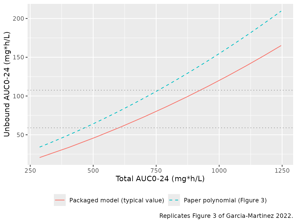
fauc_at <- approx(f3$auc_total, f3$fauc, xout = c(465, 761))$y
knitr::kable(
  tibble(
    "Total AUC0-24 (mg*h/L)" = c(465, 761),
    "Paper fAUC target" = c(59, 107.5),
    "Packaged model fAUC" = fauc_at
  ),
  digits = 1,
  caption = "Unbound AUC at the two published total-AUC anchors."
)| Total AUC0-24 (mg*h/L) | Paper fAUC target | Packaged model fAUC |
|---|---|---|
| 465 | 59.0 | 41.4 |
| 761 | 107.5 | 81.8 |
The packaged model gives unbound AUCs about 25-30% below the paper’s polynomial at the two anchors. The paper does not say how its Figure 3 curve was generated (time grid, covariate values, or whether it pooled Monte Carlo draws). Because total AUC is non-linear in the random effects, a polynomial fitted to pooled population draws over the paper’s simulation grid differs from the typical-value curve; the maintainers checked that reading too and it still gave about 52 and 83 mgh/L at the anchors, below the published 59 and 107.5. This figure is therefore not reproduced and is reported as a deviation. The probability-of-target analysis below, which uses the 107.5 mgh/L unbound target directly and depends on the same binding constants through the trough, is reproduced.
Probability of target attainment and trough safety (Figures 4-6, Table 3)
The paper simulated 10,000 patients per scenario on a grid of creatinine clearance (30, 60, 90 mL/min/1.73 m^2), body weight (50-100 kg) and mg/kg dose, and reported (A) the probability that unbound AUC / MIC >= 107.5 and (B) the probability that the total trough concentration is >= 24.3 mg/L, the threshold associated with creatine phosphokinase elevation. Here 200 sets of random effects are drawn once in R and reused across every scenario (common random numbers), so the results below are identical on every machine.
Because the unbound system is linear, the unbound AUC is proportional to dose and is computed once per renal-function level for a 100 mg reference dose; the total trough is non-linear in dose (saturable binding) and is simulated for every scenario.
set.seed(20221018)
n_mc <- 200
etas <- tibble(
  sid = seq_len(n_mc),
  etalcl = rnorm(n_mc, 0, sqrt(0.1024)),
  etalvp = rnorm(n_mc, 0, sqrt(0.2209))
)
crcl_levels <- c(30, 60, 90)
wt_levels <- seq(50, 100, by = 10)
solve_crn <- function(events) solve_typical(events, keep = c("CRCL", "scen"))
fauc_grid <- c(0, seq(0.02, 0.6, by = 0.02), seq(0.7, 2, by = 0.1), seq(2.5, 24, by = 0.5))
fauc_events <- tidyr::crossing(etas, CRCL = crcl_levels) |>
  mutate(id = row_number(), scen = paste0("CRCL ", CRCL)) |>
  tidyr::crossing(time = fauc_grid) |>
  mutate(evid = 0L, amt = NA_real_, rate = NA_real_)
fauc_events <- bind_rows(
  fauc_events |> distinct(id, sid, etalcl, etalvp, CRCL, scen) |>
    mutate(time = 0, evid = 1L, amt = 100, rate = 200),
  fauc_events
) |>
  mutate(cmt = "central") |>
  arrange(id, time, desc(evid))
sim_fauc <- solve_crn(fauc_events) |> filter(!is.na(Cunbound))
#> ℹ omega/sigma items treated as zero: 'etalcl', 'etalvp'
fauc_nca <- PKNCA::pk.nca(PKNCA::PKNCAdata(
  PKNCA::PKNCAconc(sim_fauc, Cunbound ~ time | scen + id),
  PKNCA::PKNCAdose(fauc_events |> filter(evid == 1) |> select(id, scen, time, amt), amt ~ time | scen + id),
  intervals = data.frame(start = 0, end = 24, auclast = TRUE)
))
fauc_ref <- as.data.frame(fauc_nca) |>
  filter(PPTESTCD == "auclast") |>
  select(id, auc0_24 = PPORRES) |>
  left_join(fauc_events |> distinct(id, CRCL), by = "id")
stopifnot(nrow(fauc_ref) == n_mc * length(crcl_levels), !anyNA(fauc_ref$auc0_24))
make_trough_events <- function(mgkg, interval, n_dose, t_obs) {
  tidyr::crossing(etas, CRCL = crcl_levels, WT = wt_levels, mgkg = mgkg) |>
    mutate(id = row_number(), scen = paste(CRCL, WT, mgkg, sep = "_"), dose = mgkg * WT) |>
    tidyr::crossing(dose_n = c(seq_len(n_dose), NA)) |>
    mutate(
      evid = ifelse(is.na(dose_n), 0L, 1L),
      time = ifelse(is.na(dose_n), t_obs, (dose_n - 1) * interval),
      amt = ifelse(evid == 1, dose, NA_real_),
      rate = ifelse(evid == 1, dose / 0.5, NA_real_),
      cmt = "central"
    ) |>
    arrange(id, time, desc(evid))
}
trough_of <- function(events, regimen) {
  sim <- solve_crn(events) |> filter(!is.na(Cc))
  sim |>
    select(id, Cc) |>
    left_join(events |> distinct(id, CRCL, WT, mgkg, dose), by = "id") |>
    mutate(regimen = regimen)
}
troughs <- bind_rows(
  trough_of(make_trough_events(5:12, 24, 1, 24), "q24h"),
  trough_of(make_trough_events(5:12, 12, 2, 24), "q12h"),
  trough_of(make_trough_events(10:17, 48, 1, 48), "q48h")
)
#> ℹ omega/sigma items treated as zero: 'etalcl', 'etalvp'
#> [====|====|====|====|====|====|====|====|====|====] 0:00:02
#> ℹ omega/sigma items treated as zero: 'etalcl', 'etalvp'
#> [====|====|====|====|====|====|====|====|====|====] 0:00:04
#> ℹ omega/sigma items treated as zero: 'etalcl', 'etalvp'
#> [====|====|====|====|====|====|====|====|====|====] 0:00:02
p_tox <- troughs |>
  group_by(regimen, CRCL, WT, mgkg) |>
  summarise(p_tox = mean(Cc >= 24.3), .groups = "drop")
p_tox |>
  filter(regimen == "q24h") |>
  ggplot(aes(factor(mgkg), 100 * p_tox, fill = mgkg)) +
  geom_col() +
  geom_hline(yintercept = 20, linetype = 2, colour = "grey50") +
  facet_grid(WT ~ CRCL, labeller = label_both) +
  scale_fill_gradient(low = "#a6611a", high = "#01665e", guide = "none") +
  labs(x = "Dose (mg/kg)", y = "Probability of Cmin >= 24.3 mg/L (%)",
       caption = "Replicates Figure 4B of Garcia-Martinez 2022 (q24h, trough at 24 h).")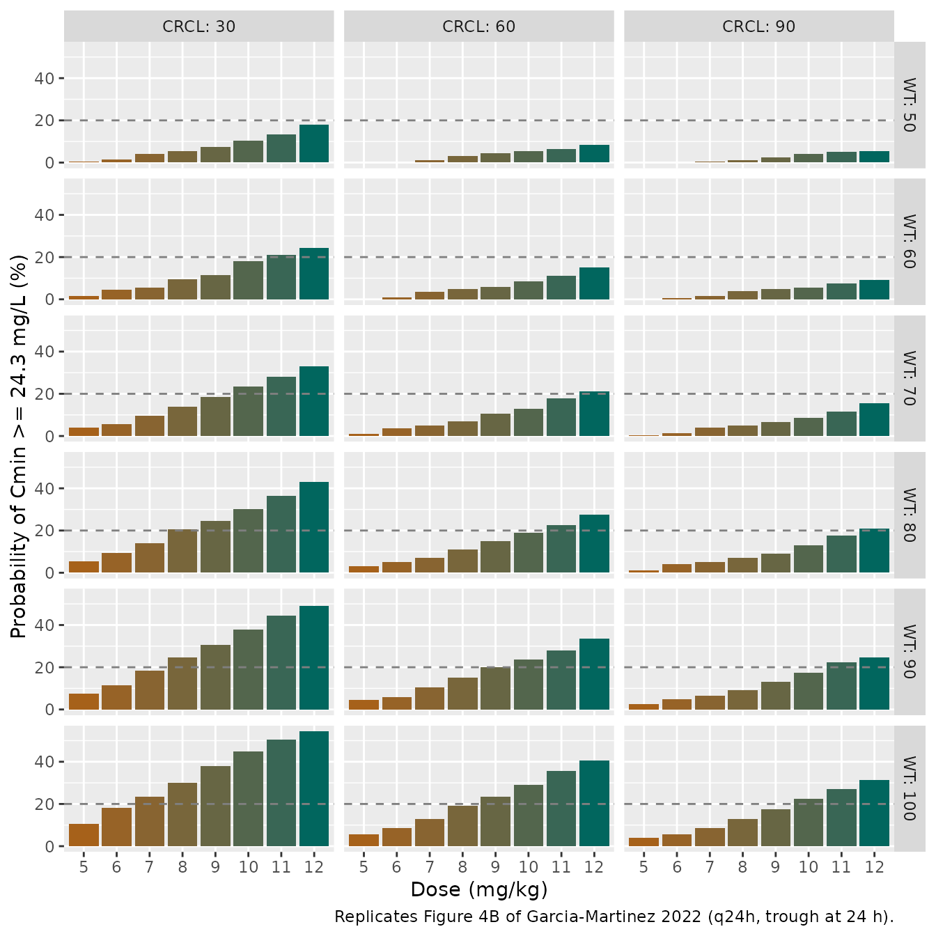
The 12 mg/kg column of Figure 4B (plus three lower-dose bars) was digitised by the maintainers and is compared with the simulation below.
fig4b <- tibble::tribble(
  ~CRCL, ~WT, ~mgkg, ~paper_pct,
  30, 50, 12, 17, 30, 60, 12, 26, 30, 70, 12, 35, 30, 80, 12, 43, 30, 90, 12, 50, 30, 100, 12, 56,
  60, 50, 12, 10, 60, 60, 12, 17, 60, 70, 12, 24, 60, 80, 12, 29, 60, 90, 12, 36, 60, 100, 12, 42,
  90, 50, 12, 7, 90, 60, 12, 12, 90, 70, 12, 17, 90, 80, 12, 22, 90, 90, 12, 28, 90, 100, 12, 34,
  30, 100, 5, 11, 30, 100, 8, 32, 60, 100, 8, 19, 90, 100, 8, 14
)
cmp4b <- fig4b |>
  left_join(filter(p_tox, regimen == "q24h"), by = c("CRCL", "WT", "mgkg")) |>
  mutate(sim_pct = 100 * p_tox, diff = sim_pct - paper_pct)
knitr::kable(
  cmp4b |>
    select(CRCL, WT, mgkg, paper_pct, sim_pct, diff) |>
    rename(
      "CRCL (mL/min/1.73 m^2)" = CRCL, "WT (kg)" = WT, "Dose (mg/kg)" = mgkg,
      "Paper (%)" = paper_pct, "Simulated (%)" = sim_pct, "Difference (points)" = diff
    ),
  digits = 0,
  caption = "P(trough >= 24.3 mg/L) after one q24h dose: Figure 4B vs simulation."
)| CRCL (mL/min/1.73 m^2) | WT (kg) | Dose (mg/kg) | Paper (%) | Simulated (%) | Difference (points) |
|---|---|---|---|---|---|
| 30 | 50 | 12 | 17 | 18 | 1 |
| 30 | 60 | 12 | 26 | 24 | -2 |
| 30 | 70 | 12 | 35 | 33 | -2 |
| 30 | 80 | 12 | 43 | 43 | 0 |
| 30 | 90 | 12 | 50 | 49 | -1 |
| 30 | 100 | 12 | 56 | 55 | -1 |
| 60 | 50 | 12 | 10 | 8 | -2 |
| 60 | 60 | 12 | 17 | 15 | -2 |
| 60 | 70 | 12 | 24 | 21 | -3 |
| 60 | 80 | 12 | 29 | 28 | -1 |
| 60 | 90 | 12 | 36 | 34 | -2 |
| 60 | 100 | 12 | 42 | 40 | -2 |
| 90 | 50 | 12 | 7 | 6 | -2 |
| 90 | 60 | 12 | 12 | 9 | -3 |
| 90 | 70 | 12 | 17 | 16 | -2 |
| 90 | 80 | 12 | 22 | 21 | -1 |
| 90 | 90 | 12 | 28 | 24 | -4 |
| 90 | 100 | 12 | 34 | 32 | -2 |
| 30 | 100 | 5 | 11 | 10 | 0 |
| 30 | 100 | 8 | 32 | 30 | -2 |
| 60 | 100 | 8 | 19 | 19 | 0 |
| 90 | 100 | 8 | 14 | 13 | -1 |
stopifnot(
  nrow(cmp4b) == 22, !anyNA(cmp4b$sim_pct),
  abs(median(cmp4b$diff)) < 5,
  max(abs(cmp4b$diff)) < 12
)
Recommended doses (Table 3)
Table 3 lists, for each renal function and body weight, the lowest dose that gives a probability of target attainment of at least 90% while keeping the probability of a toxic trough at or below 20%; an asterisk marks cells where even the top dose stays below 90% attainment. Following the paper’s Methods, the unbound AUC is the first-dose AUC0-24 for every regimen.
pta_of <- function(regimen, mgkg_grid, mic) {
  tidyr::crossing(CRCL = crcl_levels, WT = wt_levels, mgkg = mgkg_grid) |>
    rowwise() |>
    mutate(pta = {
      ref <- fauc_ref$auc0_24[fauc_ref$CRCL == CRCL]
      mean(ref * (mgkg * WT / 100) / mic >= 107.5)
    }) |>
    ungroup() |>
    mutate(regimen = regimen)
}
pta <- bind_rows(
  pta_of("q24h", 5:12, 0.5),
  pta_of("q48h", 10:17, 1)
) |>
  left_join(p_tox, by = c("regimen", "CRCL", "WT", "mgkg"))
recommend <- pta |>
  group_by(regimen, CRCL, WT) |>
  summarise(
    sim_mgkg = if (any(pta >= 0.9 & p_tox <= 0.2)) min(mgkg[pta >= 0.9 & p_tox <= 0.2]) else max(mgkg),
    sim_star = !any(pta >= 0.9 & p_tox <= 0.2),
    .groups = "drop"
  )
table3 <- tibble(
  regimen = rep(c("q24h", "q48h"), each = 18),
  CRCL = rep(rep(crcl_levels, each = 6), 2),
  WT = rep(wt_levels, 6),
  paper_mgkg = c(
    10, 9, 8, 7, 6, 5, 11, 10, 9, 7, 7, 6, 12, 10, 9, 8, 7, 6,
    17, 16, 14, 12, 11, 10, 17, 17, 16, 14, 12, 11, 17, 17, 17, 15, 13, 12
  ),
  paper_star = c(rep(FALSE, 18), TRUE, rep(FALSE, 5), TRUE, TRUE, rep(FALSE, 4), TRUE, TRUE, rep(FALSE, 4))
)
cmp3 <- table3 |>
  left_join(recommend, by = c("regimen", "CRCL", "WT")) |>
  mutate(diff = sim_mgkg - paper_mgkg)
knitr::kable(
  cmp3 |>
    mutate(
      paper = paste0(paper_mgkg, ifelse(paper_star, "*", "")),
      simulated = paste0(sim_mgkg, ifelse(sim_star, "*", ""))
    ) |>
    select(regimen, CRCL, WT, paper, simulated) |>
    rename(
      "Regimen (target MIC)" = regimen, "CRCL (mL/min/1.73 m^2)" = CRCL, "WT (kg)" = WT,
      "Table 3 (mg/kg)" = paper, "Simulated (mg/kg)" = simulated
    ),
  caption = "Lowest dose with PTA >= 90% and P(toxic trough) <= 20%; q24h at MIC 0.5 mg/L, q48h at MIC 1 mg/L. * = PTA < 90% at the top dose."
)| Regimen (target MIC) | CRCL (mL/min/1.73 m^2) | WT (kg) | Table 3 (mg/kg) | Simulated (mg/kg) |
|---|---|---|---|---|
| q24h | 30 | 50 | 10 | 10 |
| q24h | 30 | 60 | 9 | 8 |
| q24h | 30 | 70 | 8 | 7 |
| q24h | 30 | 80 | 7 | 6 |
| q24h | 30 | 90 | 6 | 6 |
| q24h | 30 | 100 | 5 | 5 |
| q24h | 60 | 50 | 11 | 11 |
| q24h | 60 | 60 | 10 | 9 |
| q24h | 60 | 70 | 9 | 8 |
| q24h | 60 | 80 | 7 | 7 |
| q24h | 60 | 90 | 7 | 6 |
| q24h | 60 | 100 | 6 | 6 |
| q24h | 90 | 50 | 12 | 12 |
| q24h | 90 | 60 | 10 | 10 |
| q24h | 90 | 70 | 9 | 9 |
| q24h | 90 | 80 | 8 | 8 |
| q24h | 90 | 90 | 7 | 7 |
| q24h | 90 | 100 | 6 | 6 |
| q48h | 30 | 50 | 17* | 17* |
| q48h | 30 | 60 | 16 | 16 |
| q48h | 30 | 70 | 14 | 14 |
| q48h | 30 | 80 | 12 | 12 |
| q48h | 30 | 90 | 11 | 11 |
| q48h | 30 | 100 | 10 | 10 |
| q48h | 60 | 50 | 17* | 17* |
| q48h | 60 | 60 | 17* | 17* |
| q48h | 60 | 70 | 16 | 16 |
| q48h | 60 | 80 | 14 | 14 |
| q48h | 60 | 90 | 12 | 12 |
| q48h | 60 | 100 | 11 | 11 |
| q48h | 90 | 50 | 17* | 17* |
| q48h | 90 | 60 | 17* | 17* |
| q48h | 90 | 70 | 17 | 17 |
| q48h | 90 | 80 | 15 | 15 |
| q48h | 90 | 90 | 13 | 13 |
| q48h | 90 | 100 | 12 | 12 |
stopifnot(
  nrow(cmp3) == 36, !anyNA(cmp3$sim_mgkg),
  mean(cmp3$diff == 0) >= 0.6,
  all(abs(cmp3$diff) <= 1)
)
The paper’s text also states that 17 mg/kg q48h in patients with CRCL >= 60 mL/min/1.73 m^2 and body weight <= 60 kg gives 60-85% attainment with a toxic trough probability below 11%, and that q12h dosing raises the toxic-trough probability well above 20%:
claims <- pta |>
  filter(regimen == "q48h", mgkg == 17, CRCL >= 60, WT <= 60)
knitr::kable(
  claims |>
    select(CRCL, WT, pta, p_tox) |>
    mutate(pta = 100 * pta, p_tox = 100 * p_tox) |>
    rename("CRCL (mL/min/1.73 m^2)" = CRCL, "WT (kg)" = WT, "PTA (%)" = pta, "P(toxic trough) (%)" = p_tox),
  digits = 0,
  caption = "17 mg/kg q48h, MIC 1 mg/L."
)| CRCL (mL/min/1.73 m^2) | WT (kg) | PTA (%) | P(toxic trough) (%) |
|---|---|---|---|
| 60 | 50 | 71 | 0 |
| 60 | 60 | 88 | 1 |
| 90 | 50 | 62 | 0 |
| 90 | 60 | 82 | 0 |
Assumptions and deviations
- IIV scale. Table 2 reports inter-individual variability as a percentage for exponential random effects without stating whether it is the standard deviation of eta or a coefficient of variation. It is encoded as the SD of eta (variance = 0.32^2 and 0.47^2). The two readings differ by under 10% in variance and cannot be told apart by the reproduced Figure 4B probabilities. The bootstrap interval printed for the V2 variability (52-94%) does not contain its own point estimate (47%) or bootstrap median (46%) and was not used.
-
Residual error. Table 2’s ‘Additive on Log-scale
(%) = 22’ is encoded as
lnorm(expSd)withexpSd = 0.22, consistent with the log-transformed observations described in Results 3.1. -
Table misprints. Table 2 prints the unit of V2 as
L/h (it is a volume; Figure 1 calls it an apparent volume). The
Discussion quotes
KD = 1.96 mg/L, which is the Q estimate; Table 2 and the Results text both give 3.56 mg/L, which is used. -
Covariate. Creatinine clearance was estimated with
the Cockcroft-Gault formula and reported in mL/min/1.73 m^2; it is
stored in the canonical
CRCLcolumn and enters unbound clearance as (CRCL / 92.8)^0.19. Equation 4 centres on 92.8; Table 1 rounds the cohort median to 93. - Simulated troughs and PTA exclude residual error, matching the paper’s Monte Carlo description (log-normal PK parameters only). The q24h trough is taken at 24 h after one dose, the q12h trough at 24 h (after the second dose), and the q48h trough at 48 h, which is the reading under which the Figure 6B probabilities stay near zero.
- Figure 3 not reproduced. The total-versus-unbound AUC curve of the packaged model sits about 25-30% below the paper’s printed polynomial; see the Figure 3 section. The Figure 4B probabilities and the Table 3 dose recommendations, which depend on the same binding constants, are reproduced.
- Virtual cohort. Creatinine clearance for the steady-state cohort was drawn log-normally from the Table 1 median and IQR and truncated to 15-200 mL/min/1.73 m^2; all patients received the cohort median dose of 675 mg.
- No correction notice for the article was found in Europe PMC as of 2026-10-10.