Enteric-coated mycophenolate sodium in paediatric renal transplant (Wang 2022b)
Source:vignettes/articles/Wang_2022b_mycophenolic_acid.Rmd
Wang_2022b_mycophenolic_acid.RmdModel and source
- Citation: Wang G, Ye Q, Huang Y, Xu H, Li Z. Population Pharmacokinetics of Enteric-Coated Mycophenolate Sodium in Children after Renal Transplantation and Initial Dosage Recommendation Based on Body Surface Area. Comput Math Methods Med. 2022;2022:1881176. doi:10.1155/2022/1881176.
- Description: Population PK model for mycophenolic acid (MPA) after oral enteric-coated mycophenolate sodium (EC-MPS) in children after renal transplantation (Wang 2022b). One-compartment disposition with linear elimination and a double extravascular absorption: a first-order arm (rate ka, fraction F of the MPA dose, lag time Tlag1) running in parallel with a zero-order arm (duration Tk02, fraction 1 - F) whose lag time Tlag2 = Tlag1 + diffTlag2 is longer than the first. The EC-MPS dose is converted to MPA by the factor 0.936. Body surface area enters the apparent clearance as a power term (BSA / 1.23)^1.30. Log-normal IIV on all seven absorption and disposition parameters; combined additive plus proportional residual error. Each oral dose is given as two event records, one to depot and one to central with rate = -2.
- Article: https://doi.org/10.1155/2022/1881176 (open access, PMC9482478)
Wang 2022 developed a population pharmacokinetic model of
mycophenolic acid (MPA) in children treated with enteric-coated
mycophenolate sodium (EC-MPS, Myfortic) after renal transplantation, and
used it to recommend initial EC-MPS regimens by body surface area (BSA).
The file carries the 2022b suffix because
Wang_2022_mycophenolic_acid is a different paper (adult
renal transplant recipients on mycophenolate mofetil).
The structural model is one compartment with linear elimination and a
“double extravascular absorption”: a first-order arm (rate
ka, fraction F of the MPA dose, lag
Tlag1) in parallel with a zero-order arm (duration
Tk02, fraction 1 - F) whose lag is longer than
the first, Tlag2 = Tlag1 + diffTlag2. The EC-MPS dose is
multiplied by 0.936 to give the MPA amount. BSA acts on clearance as
CL/F = 4.28 * (BSA / 1.23)^1.30.
Dosing the model
Each oral EC-MPS dose is two event records at the same time with the
same EC-MPS amount: one to depot (the first-order arm) and
one to central with rate = -2 (the zero-order
arm, whose duration d2 is a model parameter). The model
applies the fractions 0.936 * ffo and
0.936 * (1 - ffo) and the two lag times itself.
mod <- readModelDb("Wang_2022b_mycophenolic_acid")

# Repeated EC-MPS dosing for a cohort: one row per subject in `subj`
# (id, BSA, amt, ii), doses from time 0 to `t_last`.
make_doses <- function(subj, t_last) {
  base <- subj |>
    mutate(
      time = 0,
      evid = 1L,
      addl = as.integer(round(t_last / ii))
    )
  bind_rows(
    base |> mutate(cmt = "depot", rate = 0),
    base |> mutate(cmt = "central", rate = -2)
  )
}
Population
The modelling group was 96 children (52 boys, 44 girls) aged 13.3 years (median; range 4.3-18.0) weighing 39.0 kg (15.0-67.0), height 147 cm (102-171) and BSA 1.26 m^2 (0.66-1.78; Mosteller formula), sampled a median 396 days (13-2258) after transplantation at the Children’s Hospital of Fudan University, Shanghai (Wang 2022 Table 1). Median creatinine clearance was 78.8 mL/min/1.73 m^2. 94 children received tacrolimus and 2 cyclosporin. EC-MPS doses were 10.5 mg/kg/day (3.4-24.0), or 325 mg/m^2/day (117-605), on an unchanged regimen for at least five days before therapeutic drug monitoring. MPA was sampled 30 min before a dose and 20 min, 1 h and 3 h after it (384 concentrations) and measured by EMIT (LLOQ 0.1 mg/L). The model was fitted in Monolix 2019R1 and externally validated in 32 further children (Table 3: MPE -0.880%, MAPE 10.0%, RMSE 0.810 mg/L).
Source trace
| Model element | Value | Source |
|---|---|---|
| One-compartment model, parallel first-order + zero-order absorption | – | Methods 2.2, Figure 1, Table 2 footnote |
EC-MPS to MPA conversion fmpa
|
0.936 | Methods 2.2 |
lka (ka1) |
log(0.123) 1/h | Table 2, final model |
ld2 (Tk02) |
log(2.90) h | Table 2 |
lffo (F) |
log(0.553) | Table 2 |
ltlag (Tlag1) |
log(8.45) h | Table 2 |
ldtlag2 (diffTlag2),
tlag2 = tlag + dtlag2
|
log(5.78) h | Table 2; Table 2 footnote |
lvc (V/F) |
log(3.73) L | Table 2 |
lcl (CL/F at BSA 1.23 m^2) |
log(4.28) L/h | Table 2; Results 3.2 equation |
e_bsa_cl |
1.30 | Table 2 (theta_CL-BSA); Results 3.2 equation |
| IIV SDs (ka1, Tk02, F, Tlag1, diffTlag2, V, CL) | 0.885, 2.31, 0.513, 0.576, 0.941, 0.337, 0.481 | Table 2 (omega, SD of log-normal eta; Methods 2.2) |
addSd (a) |
0.0631 mg/L | Table 2 |
propSd (b) |
0.199 | Table 2; error model in Methods 2.2 |
The variances in ini() are the squares of the Table 2
SDs.
Typical-value profile
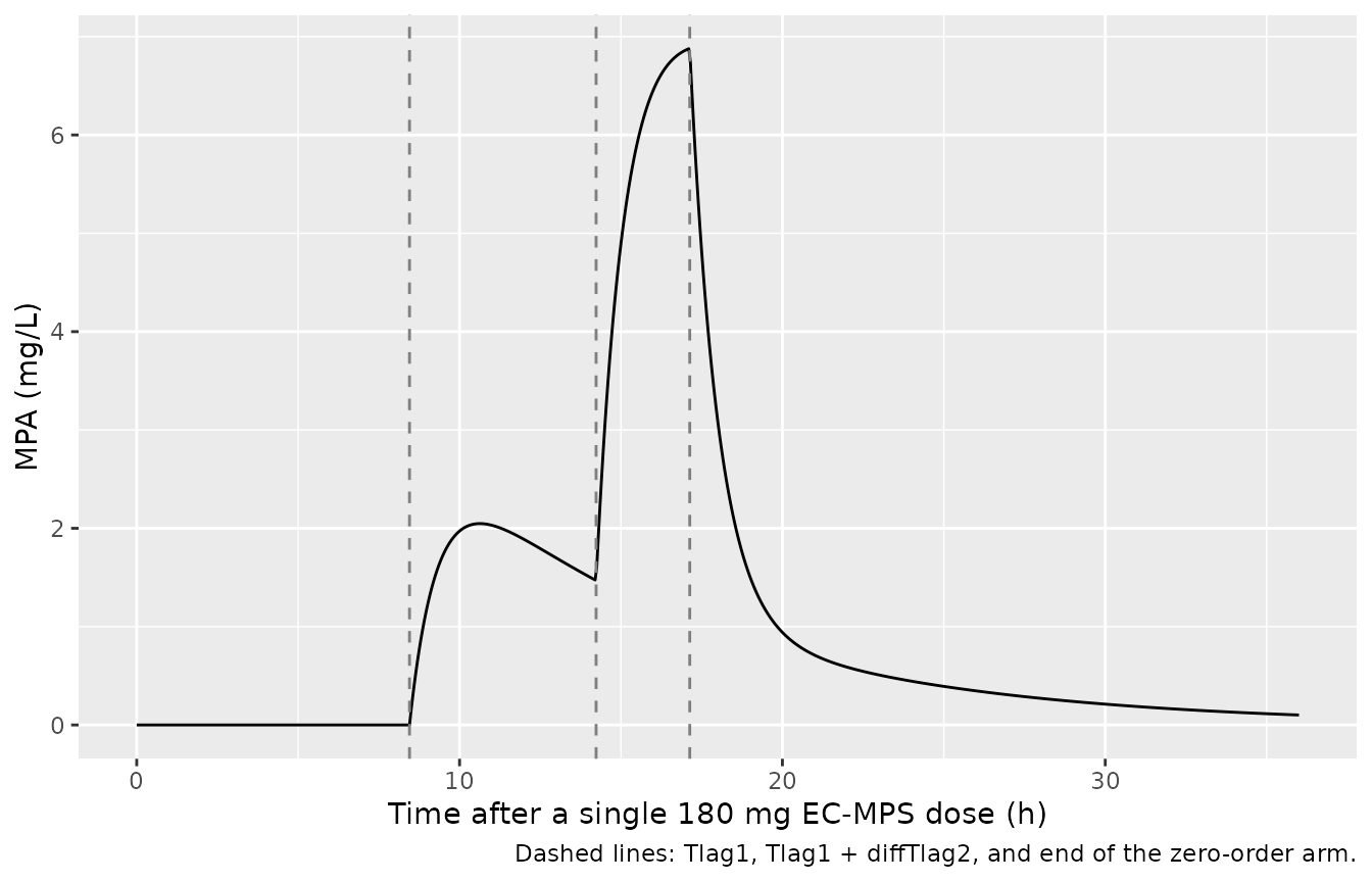
A single 180 mg EC-MPS tablet in a typical child (BSA 1.23 m^2) shows
the two absorption arms: the first-order arm starts at
Tlag1 = 8.45 h and the zero-order arm runs from
Tlag1 + diffTlag2 = 14.23 h for 2.90 h.
subj_typ <- data.frame(id = 1L, BSA = 1.23, amt = 180, ii = 24)
ev_typ <- bind_rows(
  make_doses(subj_typ, 0),
  data.frame(id = 1L, BSA = 1.23, time = seq(0, 36, by = 0.05), evid = 0L, cmt = "central")
) |>
  arrange(time, desc(evid))
sim_typ <- rxode2::rxSolve(rxode2::zeroRe(mod), events = ev_typ)
#> ℹ parameter labels from comments will be replaced by 'label()'
#> ℹ omega/sigma items treated as zero: 'etalka', 'etald2', 'etalffo', 'etaltlag', 'etaldtlag2', 'etalvc', 'etalcl'

ggplot(as.data.frame(sim_typ), aes(time, Cc)) +
  geom_line() +
  geom_vline(xintercept = c(8.45, 8.45 + 5.78, 8.45 + 5.78 + 2.90), linetype = 2, colour = "grey50") +
  labs(
    x = "Time after a single 180 mg EC-MPS dose (h)", y = "MPA (mg/L)",
    caption = "Dashed lines: Tlag1, Tlag1 + diffTlag2, and end of the zero-order arm."
  )
st <- as.data.frame(sim_typ)
# No MPA reaches plasma before the first lag time.
stopifnot(max(abs(st$Cc[st$time < 8.4])) < 1e-8)
# The zero-order arm (fraction 1 - F = 0.447 of the MPA dose) enters at
# 0.936 * 180 * 0.447 / 2.90 = 26.0 mg/h; a kink appears at its start.
d_cc <- diff(st$Cc) / diff(st$time)
i0 <- which.min(abs(st$time - 14.23))
stopifnot(d_cc[i0 + 2] - d_cc[i0 - 2] > 5)
Steady-state exposure check (PKNCA)
At steady state the dosing-interval AUC equals
0.936 * Dose / CL whatever the split between the arms, so
it checks the dose conversion, CL/F and the BSA term
together. The zero-order duration has a very wide IIV (SD 2.31 on the
log scale, so d2 exceeds 100 h in about 6% of children) and
the lags reach a day or more, so dosing runs for 40 days before the
measured interval. The cohort covers the observed BSA range on two
regimens.
The AUC uses the linear trapezoid. Children whose first-order
fraction F exceeds 1 (see “Subjects with F above 1” below)
receive a negative zero-order input, and when that input is short their
concentration dips below zero even at steady state; the log-down
trapezoid cannot integrate those intervals, while the linear trapezoid
integrates the signed concentration and still recovers the mass
balance.
rxode2::rxSetSeed(20220910)
n_per <- 40
subj_ss <- data.frame(
  id = seq_len(2 * n_per),
  BSA = rep(seq(0.66, 1.78, length.out = n_per), 2),
  amt = rep(c(180, 360), each = n_per),
  ii = 12
) |>
  mutate(treatment = paste(amt, "mg q12h"))
t_ss <- 40 * 24
obs_ss <- tidyr::crossing(
  subj_ss |> select(id, BSA, amt, ii, treatment),
  time = t_ss + seq(0, 12, by = 0.1)
) |>
  mutate(evid = 0L, cmt = "central")
ev_ss <- bind_rows(make_doses(subj_ss, t_ss), obs_ss) |>
  arrange(id, time, desc(evid))
sim_ss <- rxode2::rxSolve(mod, events = ev_ss, maxsteps = 1e6) |>
  as.data.frame()
#> ℹ parameter labels from comments will be replaced by 'label()'
conc_ss <- sim_ss |>
  filter(!is.na(Cc)) |>
  select(id, time, Cc) |>
  left_join(subj_ss |> select(id, treatment), by = "id")
dose_ss <- subj_ss |>
  mutate(time = t_ss) |>
  select(id, time, amt, treatment)
o_conc <- PKNCA::PKNCAconc(conc_ss, Cc ~ time | treatment + id)
#> Warning in assert_conc(conc, any_missing_conc = any_missing_conc): Negative
#> concentrations found
o_dose <- PKNCA::PKNCAdose(dose_ss, amt ~ time | treatment + id)
intervals <- data.frame(start = t_ss, end = t_ss + 12, auclast = TRUE, cav = TRUE)
# PKNCA warns once per subject with a negative concentration; those
# subjects are expected here (F > 1) and are counted below instead.
nca_ss <- withCallingHandlers(
  PKNCA::pk.nca(PKNCA::PKNCAdata(o_conc, o_dose, intervals = intervals, options = list(auc.method = "linear"))),
  warning = function(w) {
    if (grepl("Negative concentrations found", conditionMessage(w))) invokeRestart("muffleWarning")
  }
)
c(`Subjects with a negative Cc in the interval` = sum(tapply(conc_ss$Cc, conc_ss$id, min) < 0))
#> Subjects with a negative Cc in the interval
#>                                           6

auc_ss <- as.data.frame(nca_ss$result) |>
  filter(PPTESTCD == "auclast") |>
  select(id, treatment, auc = PPORRES) |>
  left_join(
    sim_ss |> group_by(id) |> summarise(cl = first(cl)),
    by = "id"
  ) |>
  left_join(subj_ss |> select(id, amt), by = "id") |>
  mutate(
    auc_expected = 0.936 * amt / cl,
    pct_diff = 100 * (auc / auc_expected - 1)
  )

auc_ss |>
  group_by(treatment) |>
  summarise(
    `Median AUC0-12 (mg*h/L)` = signif(median(auc), 3),
    `Median 0.936*Dose/CL (mg*h/L)` = signif(median(auc_expected), 3),
    `Median % difference` = round(median(pct_diff), 2),
    `90th pct |% difference|` = round(quantile(abs(pct_diff), 0.9), 2)
  ) |>
  dplyr::rename(Regimen = treatment) |>
knitr::kable()| Regimen | Median AUC0-12 (mg*h/L) | Median 0.936Dose/CL (mgh/L) | Median % difference | 90th pct |% difference| |
|---|---|---|---|---|
| 180 mg q12h | 47.9 | 47.9 | 0 | 0.07 |
| 360 mg q12h | 77.9 | 77.9 | 0 | 0.18 |
stopifnot(
  nrow(auc_ss) == 2 * n_per,
  !anyNA(auc_ss$pct_diff),
  # Both sides use the same drawn parameters, so the difference is
  # trapezoid error on the 0.1 h grid (largest for zero-order arms of a few
  # minutes) plus the rare subject still short of steady state after 40
  # days. Measured: median 0.005%, 90th percentile 0.09%. A mis-entered dose
  # conversion, CL/F or BSA exponent moves every subject by tens of percent.
  abs(median(auc_ss$pct_diff)) < 1,
  quantile(abs(auc_ss$pct_diff), 0.9) < 2
)
Visual predictive check (Figure 3)
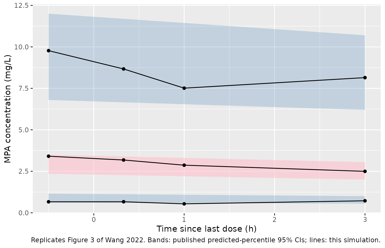
Figure 3 of Wang 2022 is a VPC of MPA concentrations at steady state against time since the last dose, at the four sampling times (-0.5, 0.33, 1 and 3 h). The doses behind it are not tabulated per child, so the virtual cohort below draws BSA from a normal distribution with mean 1.23 m^2 (the centring value of the clearance model) and SD 0.27 m^2 truncated to the observed 0.66-1.78 m^2, draws a daily dose per m^2 from a log-normal with median 325 mg/m^2/day truncated to the observed 117-605 mg/m^2/day, and rounds the twice-daily dose to whole 180 mg tablets. The model concentrations are compared with the predicted-percentile bands read from Figure 3 by the maintainers.
rxode2::rxSetSeed(2022)
n_vpc <- 200
bsa_draw <- rnorm(4 * n_vpc, 1.23, 0.27)
bsa_draw <- bsa_draw[bsa_draw >= 0.66 & bsa_draw <= 1.78][seq_len(n_vpc)]
dd_draw <- exp(rnorm(4 * n_vpc, log(325), 0.3))
dd_draw <- dd_draw[dd_draw >= 117 & dd_draw <= 605][seq_len(n_vpc)]
subj_vpc <- data.frame(
  id = seq_len(n_vpc),
  BSA = bsa_draw,
  amt = pmax(180, 180 * round(dd_draw * bsa_draw / 2 / 180)),
  ii = 12
)
t_dose <- 40 * 24
obs_vpc <- tidyr::crossing(
  subj_vpc |> select(id, BSA, amt, ii),
  tsld = c(-0.5, 0.33, 1, 3)
) |>
  mutate(time = t_dose + tsld, evid = 0L, cmt = "central") |>
  select(-tsld)
ev_vpc <- bind_rows(make_doses(subj_vpc, t_dose), obs_vpc) |>
  arrange(id, time, desc(evid))
sim_vpc <- rxode2::rxSolve(mod, events = ev_vpc, maxsteps = 1e6) |>
  as.data.frame() |>
  mutate(tsld = round(time - t_dose, 2))

table(subj_vpc$amt)
#>
#> 180 360 540
#> 162  37   1
vpc_sum <- sim_vpc |>
  group_by(tsld) |>
  summarise(
    p10 = quantile(sim, 0.1),
    p50 = quantile(sim, 0.5),
    p90 = quantile(sim, 0.9)
  )
# Predicted 95% CI bands of the 10th / 50th / 90th percentiles, read from
# Wang 2022 Figure 3 at -0.5 h and 3 h by the maintainers.
fig3 <- data.frame(
  tsld = c(-0.5, 3),
  p10_lo = c(0.60, 0.55), p10_hi = c(1.15, 1.00),
  p50_lo = c(2.35, 2.00), p50_hi = c(3.50, 3.05),
  p90_lo = c(6.80, 6.20), p90_hi = c(12.0, 10.7)
)

ggplot() +
  geom_ribbon(data = fig3, aes(tsld, ymin = p10_lo, ymax = p10_hi), fill = "steelblue", alpha = 0.25) +
  geom_ribbon(data = fig3, aes(tsld, ymin = p50_lo, ymax = p50_hi), fill = "pink", alpha = 0.6) +
  geom_ribbon(data = fig3, aes(tsld, ymin = p90_lo, ymax = p90_hi), fill = "steelblue", alpha = 0.25) +
  geom_line(data = vpc_sum |> pivot_longer(-tsld), aes(tsld, value, group = name)) +
  geom_point(data = vpc_sum |> pivot_longer(-tsld), aes(tsld, value)) +
  labs(
    x = "Time since last dose (h)", y = "MPA concentration (mg/L)",
    caption = "Replicates Figure 3 of Wang 2022. Bands: published predicted-percentile 95% CIs; lines: this simulation."
  )
knitr::kable(vpc_sum, digits = 2, caption = "Simulated percentiles of MPA (mg/L) by time since last dose.")| tsld | p10 | p50 | p90 |
|---|---|---|---|
| -0.50 | 0.66 | 3.41 | 9.77 |
| 0.33 | 0.66 | 3.18 | 8.67 |
| 1.00 | 0.54 | 2.87 | 7.51 |
| 3.00 | 0.72 | 2.50 | 8.15 |
The simulated 10th, 50th and 90th percentiles are nearly flat across the sampling window, as in Figure 3: with lags of 8 to 14 h and a slow first-order absorption (half-life 5.6 h) under 12-hourly dosing, the concentration at steady state is set by overlapping inputs from earlier doses rather than by the dose just given.
# Pooled over the four times. The cohort's doses are a reconstruction, so
# the bounds allow for it while still failing on a tenfold error in CL/F,
# V/F or the dose conversion. Robust quantiles, not extremes (cohort draws
# differ across rxode2 builds and thread counts).
pooled <- quantile(sim_vpc$sim, c(0.1, 0.5, 0.9))
pooled
#>       10%       50%       90%
#> 0.6538099 2.9559331 8.6216935
stopifnot(
  pooled[["50%"]] > 1.5, pooled[["50%"]] < 5,
  pooled[["10%"]] > 0.2, pooled[["10%"]] < 2,
  pooled[["90%"]] > 4, pooled[["90%"]] < 16
)
Subjects with F above 1
Wang 2022 states that every parameter, including the fraction
F, is log-normal. With F = 0.553 and an IIV SD
of 0.513, a child has F > 1 when
eta > log(1 / 0.553), which happens with probability
12.4%. The zero-order arm 1 - F is then negative; the total
MPA absorbed is still 0.936 times the dose. The model keeps the
published distribution.
ffo_tab <- sim_vpc |>
  group_by(id) |>
  summarise(ffo = first(ffo), min_cc = min(Cc))
c(
  `Fraction of simulated subjects with F > 1` = mean(ffo_tab$ffo > 1),
  `Fraction with any negative Cc at the sampled times` = mean(ffo_tab$min_cc < 0)
)
#>          Fraction of simulated subjects with F > 1
#>                                              0.145
#> Fraction with any negative Cc at the sampled times
#>                                              0.020
Dosing-regimen simulation (Figures 5-7)
Wang 2022 simulated 1000 children with BSA uniform on 0.22-2.03 m^2
and reported, per BSA group, the regimen with the highest percentage of
target attainment (PTA: AUC0-12 30-60 mgh/L, or the equivalent
60-120 mgh/L over 24 h and 120-240 mg*h/L over 48 h). At steady
state every one of those AUCs is
0.936 * (EC-MPS amount per 24 h) / CL scaled to its window,
so PTA depends only on the daily dose, BSA and the IIV of clearance, and
can be computed exactly:
PTA = P(60 < 0.936 * D24 / CL_i < 120) with
log CL_i ~ N(log(4.28 * (BSA / 1.23)^1.30), 0.481^2),
averaged over BSA within each group.
groups <- data.frame(
  group = c("0.22-0.46", "0.47-0.67", "0.68-0.96", "0.97-1.18", "1.19-1.58", "1.59-2.03"),
  lo = c(0.22, 0.47, 0.68, 0.97, 1.19, 1.59),
  hi = c(0.46, 0.67, 0.96, 1.18, 1.58, 2.03),
  paper_regimen = c("180 mg q48h", "180 mg q24h", "180 mg q24h", "360 mg q24h", "540 mg q24h", "360 mg q12h")
)
regimens <- tidyr::crossing(amt = c(180, 360, 540, 720), tau = c(8, 12, 16, 24, 48)) |>
  mutate(regimen = paste0(amt, " mg q", tau, "h"), d24 = amt * 24 / tau) |>
  bind_rows(data.frame(
    regimen = c("360/180 mg q12h", "540/360 mg q12h", "720/540 mg q12h"),
    d24 = c(540, 900, 1260)
  ))
pta_one <- function(d24, bsa) {
  m <- log(0.936 * d24 / (4.28 * (bsa / 1.23)^1.30))
  s <- 0.481
  pnorm((log(120) - m) / s) - pnorm((log(60) - m) / s)
}
pta_tab <- tidyr::crossing(groups, regimens) |>
  rowwise() |>
  mutate(pta = 100 * mean(pta_one(d24, seq(lo, hi, length.out = 201)))) |>
  ungroup()

pta_best <- pta_tab |>
  group_by(group) |>
  summarise(
    paper_regimen = first(paper_regimen),
    pta_paper = pta[regimen == first(paper_regimen)],
    best_pta = max(pta),
    best_regimens = paste(regimen[abs(pta - max(pta)) < 1e-9], collapse = ", ")
  )
stopifnot(nrow(pta_best) == 6, all(lengths(pta_best$pta_paper) == 1))

pta_best |>
  mutate(across(c(pta_paper, best_pta), \(x) round(x, 1))) |>
  dplyr::rename(
    `BSA group (m^2)` = group,
    `Recommended in Wang 2022` = paper_regimen,
    `PTA of that regimen (%)` = pta_paper,
    `Highest PTA (%)` = best_pta,
    `Regimen(s) with highest PTA` = best_regimens
  ) |>
knitr::kable()| BSA group (m^2) | Recommended in Wang 2022 | PTA of that regimen (%) | Highest PTA (%) | Regimen(s) with highest PTA |
|---|---|---|---|---|
| 0.22-0.46 | 180 mg q48h | 43.2 | 43.2 | 180 mg q48h |
| 0.47-0.67 | 180 mg q24h | 46.5 | 46.5 | 180 mg q24h, 360 mg q48h |
| 0.68-0.96 | 180 mg q24h | 46.7 | 48.8 | 180 mg q16h, 540 mg q48h |
| 0.97-1.18 | 360 mg q24h | 51.4 | 51.4 | 180 mg q12h, 360 mg q24h, 720 mg q48h |
| 1.19-1.58 | 540 mg q24h | 49.0 | 49.0 | 180 mg q8h, 360 mg q16h, 540 mg q24h, 360/180 mg q12h |
| 1.59-2.03 | 360 mg q12h | 50.8 | 50.8 | 360 mg q12h, 720 mg q24h |
pta_tab |>
  filter(!grepl("/", regimen)) |>
  mutate(tau = factor(paste0("q", tau, "h"), levels = paste0("q", c(8, 12, 16, 24, 48), "h"))) |>
  ggplot(aes(amt, pta, colour = group)) +
  geom_line() +
  geom_point() +
  facet_wrap(~tau) +
  labs(
    x = "EC-MPS dose (mg)", y = "PTA (%)", colour = "BSA (m^2)",
    caption = "Replicates Figure 7 (a)-(e) of Wang 2022 (exact steady-state calculation)."
  )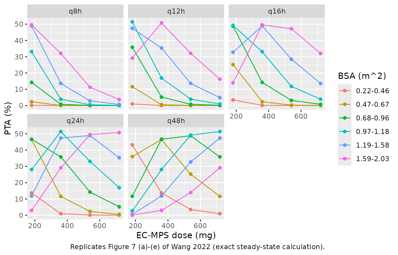
The exact calculation reproduces the paper’s recommended regimen as the best regimen in five of the six BSA groups. In the 0.68-0.96 m^2 group, 180 mg q24h (the recommendation) gives a PTA of 46.7%, against 48.8% for 270 mg/day (180 mg q16h or 540 mg q48h); with about 160 simulated children per group the paper’s Monte Carlo PTA has a standard error near 4 percentage points, so the two are not distinguishable there. The highest PTA is about 50% in every group, as the paper reports.
stopifnot(
  # The recommended regimen is (one of) the exact best in five groups.
  sum(abs(pta_best$best_pta - pta_best$pta_paper) < 1e-9) == 5,
  # Each recommended regimen is within the paper's Monte Carlo error of the best.
  all(pta_best$best_pta - pta_best$pta_paper < 5),
  # "the highest PTA among all the groups and all the dosing regimens are around 50%"
  all(pta_best$best_pta > 40 & pta_best$best_pta < 56)
)
Assumptions and deviations
-
File name.
Wang_2022_mycophenolic_acidalready holds a different Wang 2022 paper (Front Pharmacol, adult renal transplant, mycophenolate mofetil), so this model isWang_2022b_mycophenolic_acid. -
Log-normal
F. The paper states that every parameter is log-normal, including the first-order fractionF. About 12% of children then haveF > 1and a negative zero-order arm. The model keeps the published distribution rather than movingFto the logit scale, which would narrow its tails; total absorption stays 0.936 times the dose, so the steady-state AUC and the paper’s dosing recommendations are unaffected. -
Lag increment.
diffTlag2is estimated with its own IIV as the increment of the zero-order lag overTlag1; it is encoded asldtlag2, withtlag2 = tlag + dtlag2inmodel(). - BSA reference. The equation divides BSA by 1.23 m^2; the Methods centre continuous covariates on their mean, while Table 1 gives the median 1.26 m^2. The equation value is used.
-
Residual error.
Cobs = Cpred + sqrt(a^2 + (b * Cpred)^2) * epsis encoded asadd(addSd) + prop(propSd), the combined form on the variance scale. - VPC cohort. Per-child doses and BSA values are not published. The Figure 3 comparison uses a reconstructed cohort (BSA and dose per m^2 drawn to match Table 1, doses rounded to whole 180 mg tablets, 12-hourly dosing) and the predicted-percentile bands were read from the figure by eye.
- Morning and evening doses. All samples followed a morning dose, and the paper fits a single set of lag times; no diurnal difference is modelled.
-
No published NCA. The paper reports no Cmax, Tmax
or AUC table; the PKNCA check compares simulated AUC0-12 against the
steady-state identity
0.936 * Dose / CLinstead.