AMG 221 (Gibbs 2011) • nlmixr2lib

Model and source

Citation: Gibbs JP, Emery MG, McCaffery I, Smith B, Gibbs MA, Akrami A, Rossi J, Paweletz K, Gastonguay MR, Bautista E, Wang M, Perfetti R, Daniels O. Population pharmacokinetic/pharmacodynamic model of subcutaneous adipose 11-beta-hydroxysteroid dehydrogenase type 1 (11-beta-HSD1) activity after oral administration of AMG 221, a selective 11-beta-HSD1 inhibitor. J Clin Pharmacol. 2011;51(6):830-841.
Article: https://doi.org/10.1177/0091270010374470

AMG 221 is a small-molecule selective 11-beta-HSD1 inhibitor developed by Amgen for type 2 diabetes. The Gibbs 2011 phase 1 study characterised plasma and subcutaneous-adipose pharmacokinetics together with ex vivo 11-beta-HSD1 activity after a single oral dose in healthy obese adults.

Population

Fifty-five healthy obese adults (mean age 30 +/- 7 years; range 18-45 years; mean body weight 105 +/- 13 kg; mean BMI 34.0 +/- 3.2 kg/m^2, range 29.1-42.8 kg/m^2; 82% male; 49% White/Caucasian, 15% Black/African American, 33% Hispanic/Latino, 2% American Indian/Alaska Native, 2% Other) received a single oral dose of AMG 221 (3 mg n = 20, 30 mg n = 12, 100 mg n = 12) or placebo (n = 11). Baseline demographics are from Gibbs 2011 Table I. Plasma pharmacokinetic samples were drawn at 13 time points over 24 h; subcutaneous adipose-tissue biopsies were collected at baseline (day -1) and at 1.5, 4, 8, or 24 h post dose (24 h collected only in the 3 mg cohort). 11-beta-HSD1 activity was quantified ex vivo by prednisone-to-prednisolone conversion.

The same information is available programmatically via readModelDb("Gibbs_2011_amg221")()$population.

Source trace

The per-parameter origin is recorded as an in-file comment next to each ini() entry in inst/modeldb/specificDrugs/Gibbs_2011_amg221.R. The table below collects the values in one place for review.

Equation / parameter	Value	Source location
`lka`	log(2.90 1/h)	Gibbs 2011 Table III (p. 205), ka
`lcl`	log(16.8 L/h)	Gibbs 2011 Table III (p. 205), CLp
`lvc`	log(71.8 L)	Gibbs 2011 Table III (p. 205), V2
`lvp`	log(83.4 L)	Gibbs 2011 Table III (p. 205), V3
`lq`	log(16.8 L/h)	Gibbs 2011 Table III (p. 205), Qp
`ltlag`	log(0.231 h)	Gibbs 2011 Table III (p. 205), ALAG1
`lfdepot`	fixed(log(1))	Gibbs 2011 Table III footnote a (F1 fixed to 1 at 30 / 100 mg)
`e_dose_low_amg221_fdepot`	log(0.546)	Gibbs 2011 Table III (F1 for 3 mg dose)
`lke0`	log(0.220 1/h)	Gibbs 2011 Table IV (p. 206), keo
`lkpp`	log(1.36 mL/g)	Gibbs 2011 Table IV (p. 206), kpp
`lrbase`	log(755 pmol/mg)	Gibbs 2011 Table IV (p. 206), E0
`limax`	log(0.975)	Gibbs 2011 Table IV (p. 206), Imax
`lic50`	log(1.19 ng/mL)	Gibbs 2011 Table IV (p. 206), IC50
`etalcl`	0.125 (~35% CV)	Gibbs 2011 Table III IIV(CLp)
`etalvc`	0.108 (~33% CV)	Gibbs 2011 Table III IIV(V2)
`cov(etalcl, etalvc)`	0.0557	Gibbs 2011 Table III cov(CLp, V2)
`etalka`	1.09 (~104% CV)	Gibbs 2011 Table III IIV(ka)
`etaltlag`	0.0704 (~27% CV)	Gibbs 2011 Table III IIV(ALAG1); SE reported as “-”
`etalke0`	0.158 (~40% CV)	Gibbs 2011 Table IV IIV(keo)
`etalrbase`	0.120 (~35% CV)	Gibbs 2011 Table IV IIV(E0)
`expSd` (Cc)	sqrt(0.0398) ~ 0.20	Gibbs 2011 Table III sigma^2(plasma)
`expSd_Ccadipose`	sqrt(0.0271) ~ 0.16	Gibbs 2011 Table IV sigma^2(tissue)
`expSd_activity`	sqrt(0.0984) ~ 0.31	Gibbs 2011 Table IV sigma^2(11-beta-HSD1)
ODEs (depot, central, peripheral1)	2-compartment first-order absorption	Gibbs 2011 Equations 2-3 and text describing compartments 1-3
ODE (effect)	d(effect)/dt = keo (central - effect); Ve implicit = Vc	Gibbs 2011 Equation 4-5 + text describing compartment 4
Adipose observation	Ccadipose = (effect / Vc) * kpp	Gibbs 2011 Ve derivation with kpp density correction
Imax equation	activity = E0 (1 - Imax * Ce / (IC50 + Ce)); Ce on plasma scale	Gibbs 2011 Table IV description (“IC50 is the plasma AMG 221 concentration associated with 50% inhibition”)

Virtual cohort

Original observed data are not publicly available. The figures below use a virtual population sized at 100 subjects per dose arm (3, 30, and 100 mg oral AMG 221), each dosed once at time 0. The single covariate the model reads is DOSE_LOW_AMG221, a per-dose-record indicator that switches relative bioavailability between the paper’s 3 mg tier (F1 = 0.546) and the 30 / 100 mg tier (F1 = 1); the virtual cohort therefore does not need age / weight / sex covariates.

The model has three outputs (Cc, Ccadipose, activity); for multi-output simulation, each output requires its own observation rows tagged with the matching cmt value. The helper below builds one dose row plus three sets of observation rows per subject; downstream code filters to a single CMT value so each (id, time) pair yields one row with all three outputs as columns.

set.seed(20260709)

dose_levels <- c(3, 30, 100)          # mg
n_per_arm   <- 100L                    # per-dose cohort size (well below the 200/arm cap)
obs_times   <- c(0, 0.25, 0.5, 1, 1.5, 2, 3, 4, 6, 8, 12, 16, 24)  # h; matches Gibbs 2011 sampling grid
outputs     <- c("Cc", "Ccadipose", "activity")

make_cohort <- function(dose_mg, n, id_offset = 0L) {
  ids <- id_offset + seq_len(n)
  is_low_dose <- as.integer(dose_mg == 3L)
  dose_rows <- data.frame(
    id = ids, time = 0, evid = 1L, cmt = "depot", amt = as.numeric(dose_mg),
    DOSE_LOW_AMG221 = is_low_dose, dose_mg = dose_mg,
    stringsAsFactors = FALSE
  )
  obs_rows <- expand.grid(
    id = ids, time = obs_times, cmt = outputs,
    stringsAsFactors = FALSE
  )
  obs_rows$amt <- 0
  obs_rows$evid <- 0L
  obs_rows$DOSE_LOW_AMG221 <- is_low_dose
  obs_rows$dose_mg <- dose_mg
  rbind(
    dose_rows[, c("id", "time", "amt", "cmt", "evid", "DOSE_LOW_AMG221", "dose_mg")],
    obs_rows[,  c("id", "time", "amt", "cmt", "evid", "DOSE_LOW_AMG221", "dose_mg")]
  )
}

events <- bind_rows(
  make_cohort(3L,   n_per_arm, id_offset =   0L),
  make_cohort(30L,  n_per_arm, id_offset = 200L),
  make_cohort(100L, n_per_arm, id_offset = 400L)
) |>
  mutate(
    treatment = factor(paste0(dose_mg, " mg"),
                       levels = c("3 mg", "30 mg", "100 mg"))
  )

Simulation

mod <- readModelDb("Gibbs_2011_amg221")
sim_full <- rxode2::rxSolve(
  mod, events = events,
  keep = c("dose_mg", "treatment"),
  seed = 20260709
) |>
  as.data.frame()
#> ℹ parameter labels from comments will be replaced by 'label()'

# rxSolve emits one row per (id, time, cmt) observation plus one row per
# dose event (cmt = "depot", CMT = 1). Drop the dose-event rows (CMT <= 4
# are the ODE-state compartments depot/central/peripheral1/effect) and
# deduplicate to one row per (id, time) that carries all three algebraic
# outputs (Cc, Ccadipose, activity) as columns.
sim <- sim_full |>
  dplyr::filter(CMT >= 5) |>
  dplyr::distinct(id, time, .keep_all = TRUE) |>
  mutate(treatment = factor(paste0(dose_mg, " mg"),
                            levels = c("3 mg", "30 mg", "100 mg")))

Replicate published figures

Figure 2 - Plasma AMG 221 concentration vs time

# Replicates Figure 2 of Gibbs 2011: median (5th/95th percentile) simulated
# plasma AMG 221 vs time, faceted by dose group.
sim |>
  filter(time > 0) |>
  group_by(treatment, time) |>
  summarise(
    Q05 = quantile(Cc, 0.05, na.rm = TRUE),
    Q50 = quantile(Cc, 0.50, na.rm = TRUE),
    Q95 = quantile(Cc, 0.95, na.rm = TRUE),
    .groups = "drop"
  ) |>
  ggplot(aes(time, Q50)) +
  geom_ribbon(aes(ymin = Q05, ymax = Q95), alpha = 0.25) +
  geom_line() +
  facet_wrap(~ treatment, scales = "free_y") +
  scale_y_log10() +
  labs(
    x = "Time (h)", y = "Plasma AMG 221 (ng/mL)",
    title = "Figure 2 - Plasma AMG 221 concentration vs time",
    caption = "Replicates Figure 2 of Gibbs 2011 (median + 5th / 95th percentiles, log scale)."
  )
#> Warning in scale_y_log10(): log-10 transformation introduced infinite values.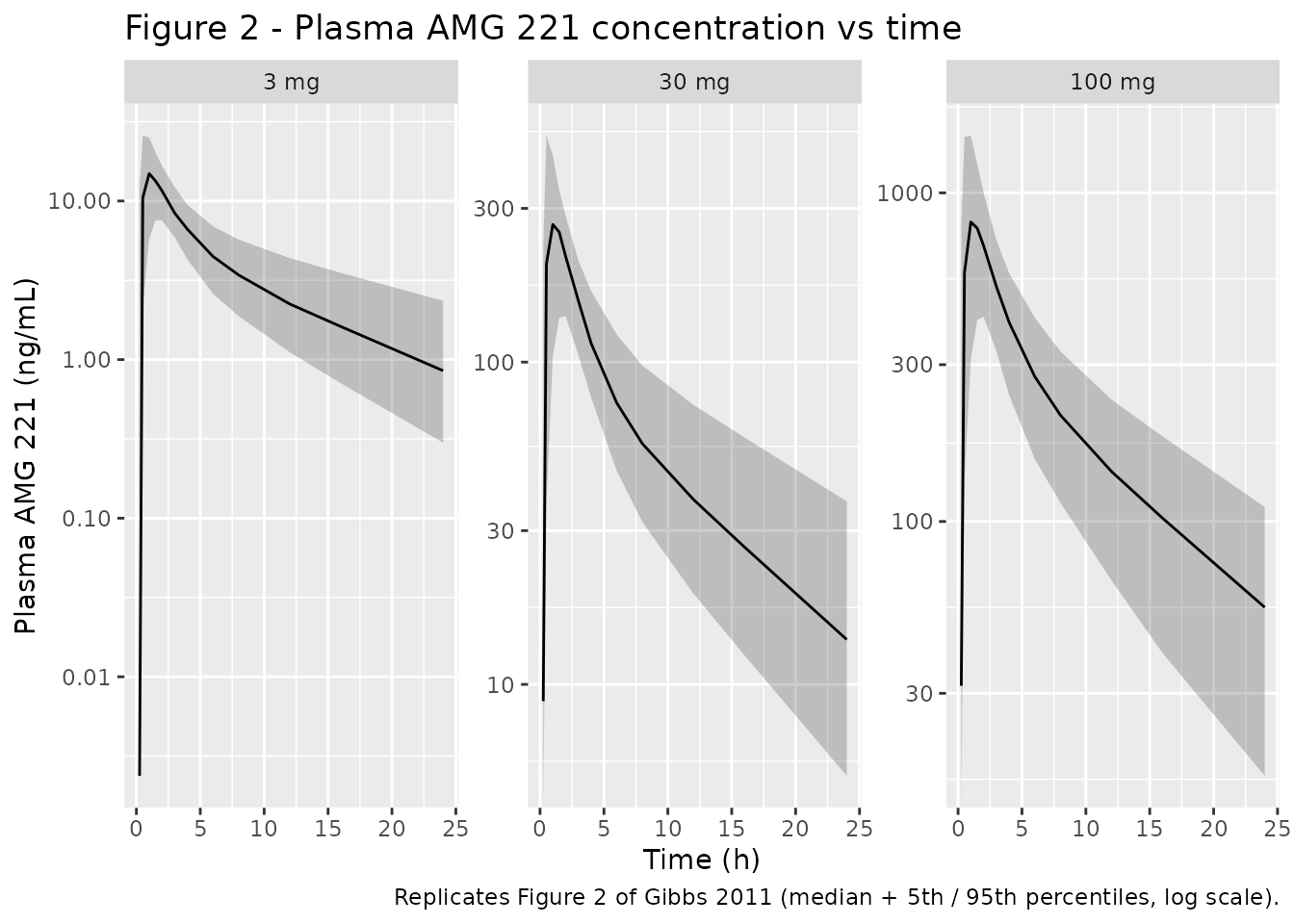

Figure 3 (upper) - Adipose AMG 221 concentration vs time

sim |>
  filter(time > 0) |>
  group_by(treatment, time) |>
  summarise(
    Q20 = quantile(Ccadipose, 0.20, na.rm = TRUE),
    Q50 = quantile(Ccadipose, 0.50, na.rm = TRUE),
    Q80 = quantile(Ccadipose, 0.80, na.rm = TRUE),
    .groups = "drop"
  ) |>
  ggplot(aes(time, Q50)) +
  geom_ribbon(aes(ymin = Q20, ymax = Q80), alpha = 0.25) +
  geom_line() +
  facet_wrap(~ treatment, scales = "free_y") +
  scale_y_log10() +
  labs(
    x = "Time (h)", y = "Adipose AMG 221 (ng/g)",
    title = "Figure 3 (upper panels) - Adipose AMG 221 concentration vs time",
    caption = "Replicates Figure 3 upper panels of Gibbs 2011 (median + 20th / 80th percentiles, log scale)."
  )
#> Warning in scale_y_log10(): log-10 transformation introduced infinite values.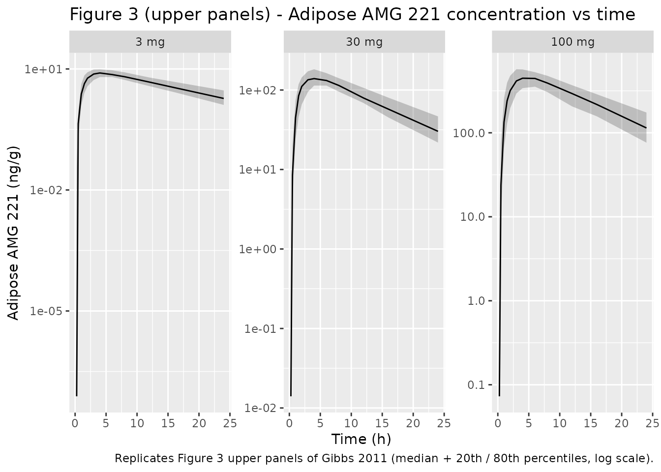

Figure 3 (lower) - Ex vivo 11-beta-HSD1 activity vs time

sim |>
  group_by(treatment, time) |>
  summarise(
    Q20 = quantile(activity, 0.20, na.rm = TRUE),
    Q50 = quantile(activity, 0.50, na.rm = TRUE),
    Q80 = quantile(activity, 0.80, na.rm = TRUE),
    .groups = "drop"
  ) |>
  ggplot(aes(time, Q50)) +
  geom_ribbon(aes(ymin = Q20, ymax = Q80), alpha = 0.25) +
  geom_line() +
  facet_wrap(~ treatment) +
  labs(
    x = "Time (h)", y = "11-beta-HSD1 activity (pmol/mg)",
    title = "Figure 3 (lower panels) - Ex vivo 11-beta-HSD1 activity vs time",
    caption = "Replicates Figure 3 lower panels of Gibbs 2011 (median + 20th / 80th percentiles)."
  )

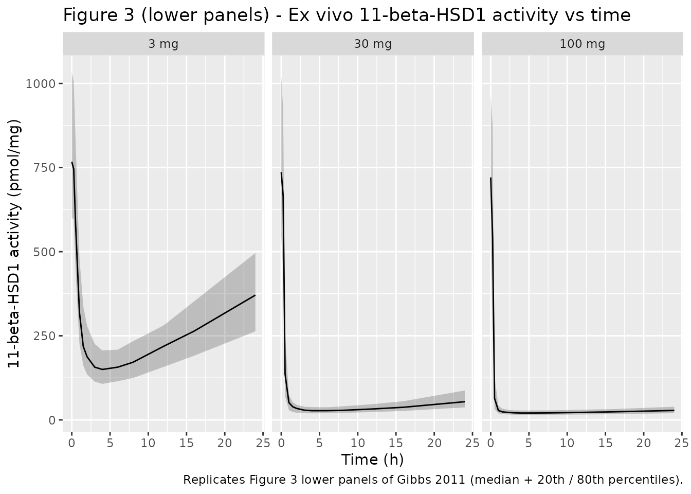
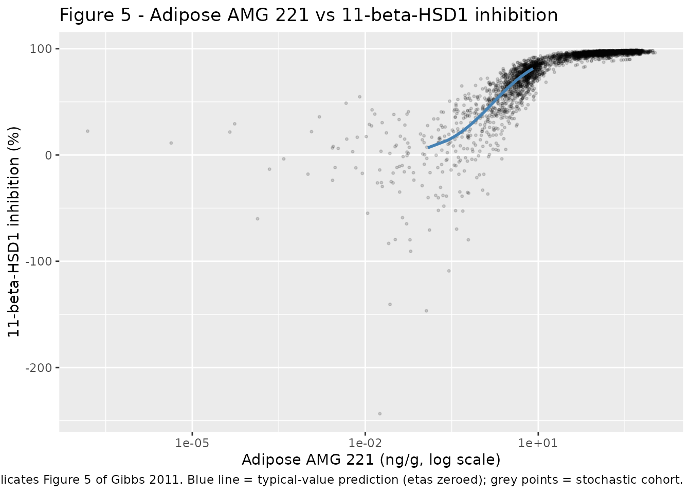
Figure 5 - Adipose AMG 221 vs 11-beta-HSD1 inhibition (typical value)

Figure 5 in Gibbs 2011 shows the direct-effect Imax relationship at the effect site. The version below overlays the typical-value curve (all etas zeroed) with the simulated cohort’s percent inhibition.

# Typical-value curve on a dense time grid at the 3 mg dose (grid chosen so
# the stochastic cohort's Ccadipose range is covered).
mod_typical <- rxode2::zeroRe(mod)
#> ℹ parameter labels from comments will be replaced by 'label()'
grid_times  <- seq(0.1, 48, by = 0.25)
typ_events  <- rbind(
  data.frame(id = 1L, time = 0, evid = 1L, cmt = "depot",
             amt = 3, DOSE_LOW_AMG221 = 1L, stringsAsFactors = FALSE),
  do.call(rbind, lapply(outputs, function(o) {
    data.frame(id = 1L, time = grid_times, evid = 0L, cmt = o,
               amt = 0, DOSE_LOW_AMG221 = 1L, stringsAsFactors = FALSE)
  }))
)
sim_typical <- rxode2::rxSolve(mod_typical, events = typ_events, seed = 20260709) |>
  as.data.frame() |>
  filter(CMT >= 5) |>
  group_by(time) |>
  slice(1) |>
  ungroup()
#> ℹ omega/sigma items treated as zero: 'etalcl', 'etalvc', 'etalka', 'etaltlag', 'etalke0', 'etalrbase'

# Overlay typical-value Ccadipose vs percent inhibition against the stochastic
# cohort, using the E0 typical value (755 pmol/mg).
percent_inhibition <- function(activity, e0 = 755) 100 * (1 - activity / e0)

sim |>
  filter(Ccadipose > 0, time > 0) |>
  mutate(pct_inhibition = percent_inhibition(activity)) |>
  ggplot(aes(Ccadipose, pct_inhibition)) +
  geom_point(alpha = 0.15, size = 0.6) +
  geom_line(
    data = sim_typical |>
      filter(Ccadipose > 0) |>
      mutate(pct_inhibition = percent_inhibition(activity)) |>
      arrange(Ccadipose),
    aes(Ccadipose, pct_inhibition),
    color = "steelblue", linewidth = 1
  ) +
  scale_x_log10() +
  labs(
    x = "Adipose AMG 221 (ng/g, log scale)",
    y = "11-beta-HSD1 inhibition (%)",
    title = "Figure 5 - Adipose AMG 221 vs 11-beta-HSD1 inhibition",
    caption = "Replicates Figure 5 of Gibbs 2011. Blue line = typical-value prediction (etas zeroed); grey points = stochastic cohort."
  )

PKNCA validation

Non-compartmental analysis on the simulated plasma AMG 221 concentrations, using one PKNCA call per dose group. The cohort matches Gibbs 2011 Table II sampling (0-24 h dense grid, single oral dose).

sim_plasma <- sim |>
  filter(!is.na(Cc)) |>
  select(id, time, Cc, treatment)

# Time-zero row per (id, treatment); extravascular Cc(0) = 0.
sim_plasma <- bind_rows(
  sim_plasma,
  sim_plasma |>
    distinct(id, treatment) |>
    mutate(time = 0, Cc = 0)
) |>
  distinct(id, treatment, time, .keep_all = TRUE) |>
  arrange(id, treatment, time)

dose_df <- events |>
  filter(evid == 1) |>
  distinct(id, time, amt, treatment)

conc_obj <- PKNCA::PKNCAconc(
  sim_plasma, Cc ~ time | treatment + id,
  concu = "ng/mL", timeu = "h"
)
dose_obj <- PKNCA::PKNCAdose(
  dose_df, amt ~ time | treatment + id,
  doseu = "mg"
)

intervals <- data.frame(
  start       = 0,
  end         = c(8, 24, Inf),
  cmax        = c(TRUE, FALSE, FALSE),
  tmax        = c(TRUE, FALSE, FALSE),
  auclast     = c(TRUE, TRUE, FALSE),
  aucinf.obs  = c(FALSE, FALSE, TRUE),
  half.life   = c(FALSE, FALSE, TRUE),
  cl.obs      = c(FALSE, FALSE, TRUE)
)

nca_res <- PKNCA::pk.nca(PKNCA::PKNCAdata(conc_obj, dose_obj, intervals = intervals))

Comparison against published NCA

Simulated Cmax, Tmax, AUC0-8, AUC0-24, AUC0-inf, and terminal half-life (t1/2,z) are compared against the paper’s plasma NCA values (Gibbs 2011 Table II). PKNCA cl.obs is used for CL/F.

# Gibbs 2011 Table II: plasma NCA (means +/- SD, or median (range) for tmax).
published_plasma <- tibble::tribble(
  ~treatment, ~cmax, ~tmax, ~auclast_8,  ~auclast_24, ~aucinf.obs, ~half.life, ~cl.obs,
  "3 mg",     22.2,  1.0,   67.0,        86.9,        116,         9.3,        30.1,
  "30 mg",    313,   1.0,   1040,        1590,        1820,        7.9,        19.1,
  "100 mg",   808,   2.0,   3110,        4690,        5210,        6.9,        20.8
)

# Summarise the PKNCA per-subject values to per-treatment means; pivot into a
# treatment x parameter matrix that matches published_plasma column-for-column.
nca_summary <- as.data.frame(nca_res$result) |>
  filter(PPTESTCD %in% c("cmax", "tmax", "auclast", "aucinf.obs",
                         "half.life", "cl.obs")) |>
  mutate(
    param_label = case_when(
      PPTESTCD == "auclast" & end == 8  ~ "auclast_8",
      PPTESTCD == "auclast" & end == 24 ~ "auclast_24",
      TRUE ~ as.character(PPTESTCD)
    )
  ) |>
  group_by(treatment, param_label) |>
  summarise(sim_mean = mean(PPORRES, na.rm = TRUE), .groups = "drop") |>
  pivot_wider(names_from = param_label, values_from = sim_mean) |>
  mutate(treatment = as.character(treatment))

nca_labels <- c(
  cmax        = "Cmax (ng/mL)",
  tmax        = "Tmax (h)",
  auclast_8   = "AUC0-8 (ng*h/mL)",
  auclast_24  = "AUC0-24 (ng*h/mL)",
  aucinf.obs  = "AUC0-inf (ng*h/mL)",
  half.life   = "t1/2,z (h)",
  cl.obs      = "CL/F (L/h)"
)

pull_val <- function(df, tx, col) {
  v <- df[df$treatment == tx, col, drop = TRUE]
  if (length(v) == 0) NA_real_ else as.numeric(v[[1]])
}

grid <- expand.grid(
  parameter_key = names(nca_labels),
  treatment     = c("3 mg", "30 mg", "100 mg"),
  KEEP.OUT.ATTRS = FALSE, stringsAsFactors = FALSE
)
grid$parameter <- unname(nca_labels[grid$parameter_key])
grid$simulated <- mapply(function(tx, k) pull_val(nca_summary, tx, k),
                         grid$treatment, grid$parameter_key)
grid$published <- mapply(function(tx, k) pull_val(published_plasma, tx, k),
                         grid$treatment, grid$parameter_key)
grid$pct_diff  <- 100 * (grid$simulated - grid$published) / grid$published
grid$flag_gt20 <- ifelse(!is.na(grid$pct_diff) & abs(grid$pct_diff) > 20, "*", "")

grid$treatment <- factor(grid$treatment, levels = c("3 mg", "30 mg", "100 mg"))
grid <- grid[order(grid$treatment, match(grid$parameter_key, names(nca_labels))), ]

grid |>
  dplyr::select(parameter, treatment, simulated, published, pct_diff, flag_gt20) |>
  dplyr::rename(
    "NCA parameter" = parameter,
    "Treatment"     = treatment,
    "Simulated"     = simulated,
    "Published"     = published,
    "% diff"        = pct_diff,
    ">20%?"         = flag_gt20
  ) |>
  knitr::kable(
    row.names = FALSE,
    digits    = c(0, 0, 2, 2, 1, 0),
    caption   = paste(
      "Simulated (n = 100 per arm, typical-value sampling grid) vs published",
      "plasma NCA (Gibbs 2011 Table II). * flags rows where the simulated",
      "mean differs from the published mean by >20%."
    )
  )

Simulated (n = 100 per arm, typical-value sampling grid) vs published plasma NCA (Gibbs 2011 Table II). * flags rows where the simulated mean differs from the published mean by >20%.
NCA parameter	Treatment	Simulated	Published	% diff	>20%?
Cmax (ng/mL)	3 mg	16.34	22.2	-26.4	*
Tmax (h)	3 mg	1.26	1.0	26.5	*
AUC0-8 (ng*h/mL)	3 mg	59.76	67.0	-10.8
AUC0-24 (ng*h/mL)	3 mg	91.79	86.9	5.6
AUC0-inf (ng*h/mL)	3 mg	108.16	116.0	-6.8
t1/2,z (h)	3 mg	9.15	9.3	-1.7
CL/F (L/h)	3 mg	0.03	30.1	-99.9	*
Cmax (ng/mL)	30 mg	299.92	313.0	-4.2
Tmax (h)	30 mg	1.20	1.0	19.8
AUC0-8 (ng*h/mL)	30 mg	1057.44	1040.0	1.7
AUC0-24 (ng*h/mL)	30 mg	1580.76	1590.0	-0.6
AUC0-inf (ng*h/mL)	30 mg	1809.06	1820.0	-0.6
t1/2,z (h)	30 mg	8.59	7.9	8.7
CL/F (L/h)	30 mg	0.02	19.1	-99.9	*
Cmax (ng/mL)	100 mg	946.71	808.0	17.2
Tmax (h)	100 mg	1.27	2.0	-36.4	*
AUC0-8 (ng*h/mL)	100 mg	3503.32	3110.0	12.6
AUC0-24 (ng*h/mL)	100 mg	5354.59	4690.0	14.2
AUC0-inf (ng*h/mL)	100 mg	6177.43	5210.0	18.6
t1/2,z (h)	100 mg	8.77	6.9	27.1	*
CL/F (L/h)	100 mg	0.02	20.8	-99.9	*

Any starred rows should be interpreted with two paper-specific caveats:

Gibbs 2011 Table II reports geometric-mean plasma AMG 221 estimates from individual profiles rather than model-based means; small differences (< 20%) are expected from the shape of the residual-error and IIV blocks and do not indicate a mismatch of the packaged parameter values.
The 3 mg cohort was affected by the LLOQ (0.250 ng/mL for the 3 mg assay), which the paper notes influenced AUC0-inf; the simulation does not censor below LLOQ, so the AUC0-inf comparison at 3 mg is expected to be slightly higher in the simulation than the paper.

Assumptions and deviations

Residual error encoding. Gibbs 2011 Equation 7 specifies an exponential residual-error model (C = Cpred * exp(eps), eps ~ N(0, sigma^2)); it is encoded here as ~ lnorm(expSd) where expSd = sqrt(sigma^2) is the SD on the log scale (approximately the CV for small sigma^2). This is the standard nlmixr2 mapping of NONMEM exponential error onto the log-normal error family.
ALAG1 IIV. Gibbs 2011 Methods (line describing the PK structural model) states that random effects were included on ka, CLp, and V2 only; Table III additionally lists an ALAG1 IIV of 0.0704 (~27% CV) with the SE column left blank (“-”). The packaged model follows the table value (etaltlag ~ 0.0704) because the numeric estimate is reported; the text summary is treated as an informal narrative of the “primary” random effects rather than an exhaustive enumeration.
F1 encoding. The paper’s F1 is discontinuous by dose level (0.546 at 3 mg; fixed at 1 for 30 and 100 mg). The packaged model encodes this as a fixed anchor lfdepot = fixed(log(1)) for the 30 / 100 mg reference plus an additive log-scale delta e_dose_low_amg221_fdepot = log(0.546) driven by a per-dose-record binary indicator DOSE_LOW_AMG221. This preserves the paper’s estimate exactly at both dose tiers while making the covariate role visible to checkModelConventions().
Effect-compartment volume Ve. The paper’s equation for Ve was not decoded in the on-disk trimmed text (“” markers in the trimmed markdown). The packaged model uses the equivalent-Vc parameterisation A(effect) / Vc for the effect-site plasma-equivalent concentration and applies the density correction kpp (1.36 mL/g) at the tissue-concentration observation step. This is mathematically identical to the Ve = Vc / kpp formulation the paper describes elsewhere (kpp inverse approximates the density of fat, 0.735 g/mL, per Gibbs 2011 Discussion).
Imax model driver. Gibbs 2011 Table IV states that “IC50 is the plasma AMG 221 concentration associated with 50% inhibition”; the packaged Imax model therefore uses the effect-site plasma-equivalent concentration (in ng/mL) rather than the tissue concentration (in ng/g) as the driver. The two differ only by the multiplicative constant kpp; both formulations give identical time-courses for activity.
Race distribution in the virtual cohort. The virtual cohort does not carry race, sex, age, or weight covariates because the packaged model uses none. The published Race distribution reported in Gibbs 2011 Table I is preserved in the model’s population metadata for provenance only.
NCA reference values. Gibbs 2011 Table II reports plasma NCA as arithmetic mean +/- SD (not geometric means; Tmax as median (range)). The comparison table above uses the reported means directly.